Programming quantum circuits

Overview
Summary
This tutorial introduces two practical ways to program quantum circuits for teaching and learning: using a visual drag‑and‑drop interface and writing code with Qiskit. You will learn how to build, visualise, and run simple quantum circuits on simulators or real quantum computers, with step‑by‑step guidance for IBM Quantum and IQM platforms. The focus is on hands‑on experimentation that is accessible for classroom use and teacher training.
Author(s): Christian Datzko (CH), Jörg Gutschank (DE)
This tutorial is part of the teaching material Quantum Computing in STEM Education.
Programming quantum circuits
Quantum circuits can be programmed by simply dragging and dropping the corresponding quantum gates in a designated field.
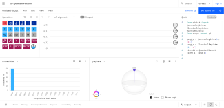
In the case of the IBM Quantum Composer, operations are dragged from a set of operations at the top left into the field in the middle of the screen. The number of qubits and the number of classical bits for the quantum circuit can be set under <Edit>–<Manage Registers>. The probability and the state of the system are predicted at the bottom of the screen, and export options – for example to Qiskit – are offered on the right.
You can run your circuit on a real IBM quantum computer if you have an account and are logged in. If not, you can use the built-in simulator, which runs the circuit on a classical computer and shows what would happen in an ideal, noise-free quantum system.[1]
How to use Qiskit to run a programme on a quantum computer
Quantum computers may also be programmed with Qiskit. Qiskit is an open source quantum computing framework that allows creating a quantum circuit by typing code lines instead of clicking on visual elements in a graphical interface. The latter can become confusing with larger quantum circuits. Qiskit provides Python modules that can be used on almost any computer. Qiskit not only provides a framework to access real quantum computers, but also to simulators and other useful tools like graphics generation.
Depending on the provider, the ways to access real quantum hardware differ slightly. Below, you find information on how to access quantum computers at IQM, a Finnish quantum hardware provider and at IBM Quantum.
Although a dedicated Python environment is not strictly necessary to run a single example, we use Miniforge to create a clearly defined and isolated Python environment. This is particularly useful for teachers who wish to experiment with both IBM Quantum and IQM backends, as these platforms may, at times, rely on different Python versions or package dependencies.
Access quantum computers at IQM
- Install Miniforge for your computer platform in order to create a clearly defined Python environment.
https://conda-forge.org/miniforge/
Create a Python environment using Python version 3.11 (sic!)[2] with the name iqm (for instance) and activate it:
conda create --name iqm python=3.11
conda activate iqm
Install the IQM client software that includes also Qiskit:
pip install "iqm-client[qiskit]"
Note the double quotation marks, without which the installation will not work on a unix or linux shell like zsh or bash.
It might also be useful to further install the python packages numpy, scipy, matplotlib, pylatexenc, and qiskit-aer with:
pip install numpy scipy matplotlib pylatexenc qiskit-aer- Create an account at IQM following this link:
https://resonance.meetiqm.com/sign-up/scienceonstage
- Navigate to your profile, create and copy your API token from there.
Run the file connection_test_iqm.py (download the file)
python connection_test_iqm.py
When you are asked for your API token paste it onto the command line and hit enter. The reply IQM backend shows that you successfully connected to IQM. If you prefer, you can also store your API token in advance (for example as an environment variable) so that you do not need to enter it interactively each time (as shown at the end of this introduction in “Creating a simple quantum circuit – Example using IBM”).
Optional: Run the file 1plus1_iqm.py (download the file)
python 1plus1_iqm.py
This program uses a quantum computer to add one and one. Decide for yourself if it is a good idea to use a quantum computer for this task.
- Optional: Install Visual Studio Code (https://code.visualstudio.com) as a graphical frontend.
The above procedure is an installation that works on almost any computer with an internet connection. You may of course use different frontends or so-called Jupyter Notebooks as you prefer.
Access quantum computers at IBM Quantum
- Install Miniforge for your computer platform in order to create a clearly defined Python environment.
https://conda-forge.org/miniforge/
Create a Python environment with the name ibm (for instance) and activate it:
conda create --name ibm python
conda activate ibm
Install Qiskit (see https://quantum.cloud.ibm.com/docs/en/guides/install-qiskit):
pip install qiskit
pip install qiskit-ibm-runtime
It might also be useful to further install the python packages numpy, scipy, matplotlib, pylatexenc, and qiskit-aer.
- Create an account at IBM following this link:
https://quantum.cloud.ibm.com/docs/en/guides/cloud-setup
Note: If you want permanent accounts for your students that do not require to give credit card numbers to IBM after a short trial period, you and every student need a so-called IBM cloud feature code before the account is created. You can get such a code with an academic institution email address only. If in doubt, use a trial account with a separate email address or ask for help at IBM beforehand.
- Create and copy your API token from here:
https://cloud.ibm.com/iam/apikeys
Make sure to directly copy the token after you have created it. The token has 44 characters. When trying to copy it later on, only 43 of the 44 characters are left!
- Copy your instance (starts with crn:) from here:
https://quantum.cloud.ibm.com/instances
Run the file connection_test_ibm.py (download the file)
python connection_test_ibm.py
When you are asked for your API token paste it into the command line and hit enter. Paste in your instance when you are asked for it and hit enter. A reply starting with ibm_ shows that you successfully connected to IBM. If you prefer, you can also store your API token in advance (for example as an environment variable) so that you do not need to enter it interactively each time (as shown at the end of this introduction in “Creating a simple quantum circuit – Example using IBM”)
Optional: Run the file 1plus1_ibm.py (download the file)
python 1plus1_ibm.py
This program uses a quantum computer to add one and one. Decide for yourself if it is a good idea to use a quantum computer for this task.
- Optional: Install Visual Studio Code (https://code.visualstudio.com) as a graphical frontend.
The above procedure is an installation that works on almost any computer with an internet connection. You may of course use different frontends or so-called Jupyter Notebooks as you prefer.
Creating a simple quantum circuit
To create a simple quantum circuit, you have to go through three steps: prepare and initialise the system, assemble the quantum circuit and optimise and execute the quantum circuit.
In the following examples, the same basic quantum operation is used in two different programming environments: a Pauli‑X gate applied to a single qubit. Although the code looks different in each case, it describes the same underlying operation. Differences in names, commands, or structure are often a matter of notation or programming style rather than a difference in quantum functionality.
import os
import getpass
from qiskit import transpile
from qiskit import QuantumCircuit, QuantumRegister, ClassicalRegister
from iqm.qiskit_iqm import IQMProvider

token = getpass.getpass("input IQM API Token: ")
os.environ["IQM_TOKEN"] = token

provider = IQMProvider(
    url="https://resonance.meetiqm.com/",
    # quantum_computer="sirius"
    # quantum_computer="garnet"
    quantum_computer="emerald"
)

backend = provider.get_backend()

qubit_register = QuantumRegister(4, 'q')
bit_register = ClassicalRegister(2, 'c')
qcirc = QuantumCircuit(qubit_register, bit_register)

# setting the input values:
# applying Pauli-X to set a=1
qcirc.x(qubit_register[0])
# applying Pauli-X to set b=1
qcirc.x(qubit_register[1])

# applying quantum gates:
# Toffoli gate
qcirc.ccx(qubit_register[0], qubit_register[1], qubit_register[3])
# CNOT
qcirc.cx(qubit_register[0], qubit_register[1])
# Toffoli
qcirc.ccx(qubit_register[1], qubit_register[2], qubit_register[3])
# CNOT
qcirc.cx(qubit_register[1], qubit_register[2])

# measure qubits 2 and 3
qcirc.measure(qubit_register[2], bit_register[0])
qcirc.measure(qubit_register[3], bit_register[1])

qcirc_transpiled = transpile(qcirc, backend)
job = backend.run(qcirc_transpiled, shots=1024)

print("job id: ", job.job_id())

result = job.result()
counts = result.get_counts()

print(
    "1 + 1 was measured 1024 times. The results are displayed as a binary number followed by the absolute frequency of the respective result."
)
print(counts)
# Create a quantum circuitfrom qiskit import QuantumRegister, ClassicalRegister, QuantumCircuit# Optimise the quantum circuitfrom qiskit.transpiler.preset_passmanagers import generate_preset_pass_manager# Access IBM Quantumfrom qiskit_ibm_runtime import QiskitRuntimeService, SamplerV2 as Sampler
service = QiskitRuntimeService(channel="ibm_quantum", token="Insert your API token here, see Profile Settings -> API token")# Choose the least busy quantum computer as backendbackend = service.least_busy(operational=True, simulator=False) # Create a sampler, that will run the job on the chosen backendsampler = Sampler(backend)# Create a pass manager that will optimise the quantum circuit for the chosen backend; optimisation level 3 is the highest possible level. Lower levels are easier to understand but produce less accurateresultspassmanager = generate_preset_pass_manager(3, backend=backend)
# One quantum register is required.quantum_registers = QuantumRegister(1, 'q')# One classical register is required.classical_registers = ClassicalRegister(1, 'c') # Both registers are added to the quantum circuit.circuit = QuantumCircuit(quantum_registers, classical_registers)# The Pauli-X gate is applied to the quantum register.circuit.x(quantum_registers[0])# A measurement is performed on the quantum register and the result is “delivered” to the classical register.circuit.measure(quantum_registers[0], classical_registers[0])
# Create the optimised quantum circuitoptimized_circuit = passmanager.run(circuit)
# Add the quantum circuit as a job to the job queuejob = sampler.run([optimized_circuit], shots=1000)# Print the Job IDprint("job id:", job.job_id())# Wait for the results; this can take some time, but the results will also be available on the IBM Quantum platform if the job is interruptedresult = job.result()print(result[0].data.c.get_counts())
The code above includes a so-called transpiler that optimises the quantum circuit. This is necessary because real quantum computers do not always offer all the desired gates. Some optimisations also reduce the quantum circuit’s noise and achieve better results.
Different ways to display quantum circuits visually using Qiskit
In addition to executing quantum circuits, Qiskit also offers the option to show quantum circuits in other representations, e.g. instead of executing the circuit, it can be visualised as text, as LaTeX source code or as image file (pixel graphics or vector graphics). Additional formats may be found at https://docs.quantum.ibm.com/api/qiskit/qiskit.visualization.circuit_drawer
# Import register:
from qiskit import QuantumRegister, ClassicalRegister, QuantumCircuit
# For output in LaTeX or as an image:
from qiskit.visualization import circuit_drawer
# For output as a matrix:
from qiskit.quantum_info import Operator
# Prepare the qubits:
quantum_registers = QuantumRegister(1, 'q')
# Prepare the bits:
classical_registers = ClassicalRegister(1, 'c')
# Create a quantum circuit:
circuit = QuantumCircuit(quantum_registers, classical_registers)
# Add a measurement:
circuit.measure(quantum_registers[0], classical_registers[0])
# Output as text:
print("The quantum circuit:")
print(circuit)
print("----------")
# Output in LaTeX:
print("The quantum circuit in LaTeX code:")
circuit_image = circuit_drawer(circuit, output="latex_source")
print(circuit_image)
print("----------")
# Output as image:
print("The quantum circuit as an image, saved as Example.png and Example.svg.")
circuit_image = circuit_drawer(circuit, output="mpl")
circuit_image.savefig("Example.png") # saved as pixel graphics
circuit_image.savefig("Example.svg") # saved as vector graphics
print("----------")A quantum circuit can also be represented as a matrix that is being applied to one or more qubits that are represented as vectors (or kets). However, this representation does not allow to include measurements. Measurements irreversibly collapse the quantum state and produce random classical results.
The following example shows a quantum circuit with a Hadamard gate
# Prepare the qubits:
quantum_registers = QuantumRegister(1, 'q')
# Prepare the bits:
classical_registers = ClassicalRegister(1, 'c')
# Create a quantum circuit:
circuit = QuantumCircuit(quantum_registers, classical_registers)
circuit.h(quantum_registers[0])
# Matrix output as text
print("The matrix is (text):")
circuit_operator = Operator.from_circuit(circuit)
print(circuit_operator.draw("text"))
print("----------")
# Matrix output
print("The matrix is (LaTeX code):")
circuit_operator = Operator.from_circuit(circuit)
print(circuit_operator.draw("latex_source"))IQM is only compatible with Python 3.11.
https://docs.quantum.ibm.com/migration-guides/local-simulators
Teaching Materials
Share this page