Mathematical Introduction: Vectors

Required materials

• paper and pencil

What is a vector?

Properties

• A vector has both a magnitude and a direction.
• The zero vector has no direction and its magnitude is 0.
• Equal vectors have the same magnitude and direction.
• A vector is usually denoted by a letter with an arrow on top like so: ${\displaystyle \stackrel{\to <!--\; \to \; -->}{v}}$. Other notations are commonly used too, such as v, v, v̄.

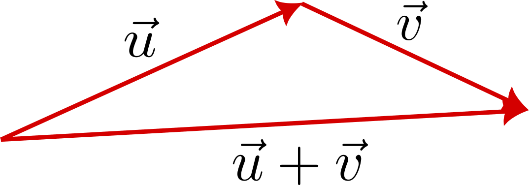
Geometrical representation of a vector

Adding two vectors geometrically is done by placing the tail of the second vector at the head of the first vector. The resulting vector starts from the tail of the first vector and ends at the head of the second vector. This method can be applied to any number of vectors.

Coordinate representations of a vector

A vector can also be represented in a standard coordinate system. In two dimensions, a vector ${\displaystyle \stackrel{\to <!--\; \to \; -->}{v}}$ can be written as a row vector, ${\displaystyle \stackrel{\to <!--\; \to \; -->}{v}=(x,y)}$, or as a column vector, ${\displaystyle \stackrel{\to <!--\; \to \; -->}{v}=\left[\begin{array}{c}x\\ y\end{array}\right]}$.
In both cases, ${\displaystyle x}$ and ${\displaystyle y}$ can be real or complex numbers.

A row vector is just the sideways version of a column vector. To switch between a row vector and a column vector, one uses the so-called transposition operation, denoted by T:
${\displaystyle (x,y{)}^T=\left[\begin{array}{c}x\\ y\end{array}\right]}$

Basic vector operations

Addition

For two vectors ${\displaystyle \stackrel{\to <!--\; \to \; -->}{u}=(x_1,y_1)}$ and ${\displaystyle \stackrel{\to <!--\; \to \; -->}{v}=(x_2,y_2)}$

${\displaystyle \stackrel{\to <!--\; \to \; -->}{u}+\stackrel{\to <!--\; \to \; -->}{v}=(x_1,y_1)+(x_2,y_2)=(x_1+x_2,y_1+y_2)}$

Subtraction

For two vectors ${\displaystyle \stackrel{\to <!--\; \to \; -->}{u}=(x_1,y_1)}$ and ${\displaystyle \stackrel{\to <!--\; \to \; -->}{v}=(x_2,y_2)}$

${\displaystyle \stackrel{\to <!--\; \to \; -->}{u}-<!--\; -\; -->\stackrel{\to <!--\; \to \; -->}{v}=(x_1,y_1)-<!--\; -\; -->(x_2,y_2)=(x_1-<!--\; -\; -->x_2,y_1-<!--\; -\; -->y_2)}$

Scalar multiplication

Multiplying a vector by a number (scalar) scales its magnitude without changing its direction (unless the scalar is negative, which also reverses its direction).

For a vector ${\displaystyle \stackrel{\to <!--\; \to \; -->}{u}=(x_1,x_2)}$ and a scalar ${\displaystyle k}$, scalar multiplication yields:

${\displaystyle k\stackrel{\to <!--\; \to \; -->}{u}=k(x_1,x_2)=(k{x}_1,k{x}_2)}$

Dot product (also called scalar product)

A way to multiply two vectors to produce a scalar is called dot (or scalar) product. For two vectors ${\displaystyle \stackrel{\to <!--\; \to \; -->}{u}=(x_1,y_1)}$ and ${\displaystyle \stackrel{\to <!--\; \to \; -->}{v}=(x_2,y_2)}$, their dot product is

${\displaystyle \stackrel{\to <!--\; \to \; -->}{u}\cdot <!--\; \cdot \; -->\stackrel{\to <!--\; \to \; -->}{v}=(x_1,y_1)\cdot <!--\; \cdot \; -->(x_2,y_2)=x_1\cdot <!--\; \cdot \; -->x_2+y_1\cdot <!--\; \cdot \; -->y_2}$

If the dot product of two vectors is zero, ${\displaystyle \stackrel{\to <!--\; \to \; -->}{u}\cdot <!--\; \cdot \; -->\stackrel{\to <!--\; \to \; -->}{v}=0}$, the two vectors are perpendicular.

Magnitude (or norm) of a vector

The magnitude of a vector ${\displaystyle \stackrel{\to <!--\; \to \; -->}{u}=(x_1,y_1)}$

${\displaystyle \Vert <!--\; \Vert \; -->\stackrel{\to <!--\; \to \; -->}{u}\Vert <!--\; \Vert \; -->=\sqrt{x_1^2+y_1^2}}$

The angle ${\displaystyle \mathrm{\theta <!--\; \theta \; -->}}$ between the two vectors can be determined as follows:

${\displaystyle \stackrel{\to <!--\; \to \; -->}{u}\cdot <!--\; \cdot \; -->\stackrel{\to <!--\; \to \; -->}{v}=\Vert <!--\; \Vert \; -->\stackrel{\to <!--\; \to \; -->}{u}\Vert <!--\; \Vert \; -->\Vert <!--\; \Vert \; -->\stackrel{\to <!--\; \to \; -->}{v}\Vert <!--\; \Vert \; -->\cos <!--\; \; -->\mathrm{\theta <!--\; \theta \; -->}}$, thus:

${\displaystyle \mathrm{\theta <!--\; \theta \; -->}=\arccos <!--\; \; -->(\stackrel{\to <!--\; \to \; -->}{u}\cdot <!--\; \cdot \; -->\stackrel{\to <!--\; \to \; -->}{v})}$

Calculating with vectors – examples

Vectors in quantum computing

Formally, the state of a qubit is a unit vector in ${\displaystyle {\mathbb{C}}^2}$, the two-dimensional complex vector space.

A single qubit can be represented by a 2-dimensional complex vector ${\displaystyle |\mathrm{\psi <!--\; \psi \; -->}⟩=\mathrm{\alpha <!--\; \alpha \; -->}|0⟩+\mathrm{\beta <!--\; \beta \; -->}|1⟩}$, where ${\displaystyle \mathrm{\alpha <!--\; \alpha \; -->}}$ and ${\displaystyle \mathrm{\beta <!--\; \beta \; -->}}$ are complex numbers satisfying ${\displaystyle {\left|\mathrm{\alpha <!--\; \alpha \; -->}\right|}^2+{\left|\mathrm{\beta <!--\; \beta \; -->}\right|}^2=1}$, and ${\displaystyle |0⟩=\left[\begin{array}{c}1\\ 0\end{array}\right]}$ and ${\displaystyle |1⟩=\left[\begin{array}{c}0\\ 1\end{array}\right]}$.

For example, the state ${\displaystyle |\mathrm{\psi <!--\; \psi \; -->}⟩=\frac{1}{\sqrt{2}}|0⟩+\frac{1}{\sqrt{2}}|1⟩}$ can be represented by the vector ${\displaystyle \frac{1}{\sqrt{2}}\left[\begin{array}{c}1\\ 1\end{array}\right]}$

or the state ${\displaystyle |\mathrm{\psi <!--\; \psi \; -->}⟩=\frac{1}{\sqrt{2}}|0⟩+\frac{1}{\sqrt{2}}i|⟩}$ can be represented by the vector ${\displaystyle \frac{1}{\sqrt{2}}\left[\begin{array}{c}1\\ i\end{array}\right]}$.

Task for students: Quiz

You can download the quiz for students here:

• Quiz as docx
• Quiz as pdf

Below you find the same questions in an interactive format.
Use this link to send the interactive H5P task to your students.