How to implement Deutsch’s algorithm with a Mach–Zehnder interferometer

Let us link theory and experiment with an additional idea connecting two teaching units of our material:

The algorithm that is taught in the lesson "Deutsch's algorithm - Mathematical approach" can be implemented with the help of a Mach–Zehnder interferometer which is introduced in the teaching unit "Light crossroads - Optical Quantum Gates in a Mach–Zehnder interferometer". The following description assumes that you are a teacher who is familiar with the two teaching units, i.e. you know how a Mach–Zehnder interferometer and Deutsch's algorithm work and are eager to go the next step.

There are two ways to do this: a one-qubit version implementing only the upper qubit $q_0$, and a two-qubit version implementing the complete algorithm with both qubits. We will explain the one-qubit version, which merely requires a simple Mach–Zehnder interferometer and two retarders¹ and point you to the literature for the two-qubit version.

Figure 1 shows Deutsch’s algorithm with the situation that the ’black box’ contains no further quantum gates (as it would be the case for the function constant zero). Let us go through quantum circuit from left to right to recall what happens.

We name the upper qubit $q_0$ and the lower qubit $q_1$, both are in the state $\text{|0⟩}$ at the beginning. $q_1$ is ’swapped’ to make it $\text{|1⟩}$.

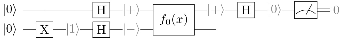
Figure 1: Quantum circuit implementing Deutsch’s algorithm. The function in the ’black box’ is constant zero, so that all the state vectors can be shown for concreteness. The upper qubit is $q_0$, the lower $q_1$.

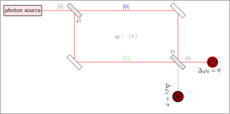
Figure 2: Mach–Zehnder interferometer implementing the qubit $q_0$ of Deutsch’s algorithm. The function in the ‘black box’ is assumed to be constant zero.

The following Hadamard gates create superpositions: $\text{|+⟩}=\frac{\text{|0⟩}+\text{|1⟩}}{\sqrt{2}}$ and $\text{|−⟩}=\frac{\text{|0⟩}-\text{|1⟩}}{\sqrt{2}}$. Behind the ‘black box’ we are merely interested in the upper qubit. For constant functions, $q_0$ is in the $\text{|+⟩}$ state, while for balanced functions, it would be in the $\text{|−⟩}$ state. The final Hadamard gate returns $\text{|0⟩}$ for constant functions while it returns $\text{|1⟩}$ for balanced functions. A measurement mainly results in zeros or ones according to whether we are dealing with a constant or a balanced function.

Each photon going through a Mach–Zehnder interferometer behaves like $q_0$, as figure 2 shows. The state at the beginning is $\text{|0⟩}$(input from the top would, for instance, yield $\text{|1⟩}$). The first beam splitter is acting like a Hadamard gate^[2] , so that the unlocalised photon is in a superposition of its ‘which-way-information’. The second beam splitter is acting like another Hadamard gate, ‘deviating’ the photon to the output at the right-hand side. We name this output $\text{|0⟩}$. For a beam of laser light we would have an interference pattern which is inverted relative to the other output, so that we could take some spot (say middle) for the measurement.

In order to implement the function $f\left(x\right)$, we need two half-wave retarders, which we use, or do not use in the upper (for $f\left(0\right)$) or lower (for $f\left(1\right)$) arm of the Mach-Zehnder interferometer. Using the retarder in the upper arm sets $f\left(0\right)=1$, using it in the lower arm sets $f\left(1\right)=1$. It is left to the interested reader to show that the result for constant functions is always the output $\text{|0⟩}$ to the right, while the result for balanced functions is the downward output.

The two-qubit version of this implementation^[3] uses two qubits in each photon. One qubit is the polarisation of the photon, i.e. spin angular momentum, the other one corresponds to two spatial modes ( $\text{TEM₁₀}$ and $\text{TEM₀₁}$) of the laser, i.e. orbital angular momentum. The details of this exciting experiment are beyond the scope of this short description.