The Bernstein-Vazirani Algorithm - Computational Approach

Overview
Overview
Keywords: Bernstein‑Vazirani algorithm, hidden binary string, Hadamard gates, ⊕-Gate, single query
Age group: 16-18 years
Required knowledge/skills: Students should have done Lesson 2 about Deutsch's algorithm
Time frame: 60 minutes
Author: Wolfgang Geist (CH)
Learning objectives
The goal of this part of the lesson is for students to deepen their understanding of the Bernstein‑Vazirani algorithm by analyzing its quantum implementation.
By working through a low‑dimensional example, students focus on how the sequence of quantum gates leads to the measurement of the hidden string and how this result can be generalized to larger input sizes.
Additional tool for Bernstein-Vazirani lesson
The spreadsheet tool can be used to model any 3‑qubit Bernstein‑Vazirani problem and to illustrate the basic set‑up of the function and the underlying circuitry. By using Hadamard gates, it shows how the hidden string can be determined, and the coefficients may be hidden so that students can attempt to deduce the string themselves.
The tool is designed for teacher‑led exposition prior to the exercises in the lesson. While it can be configured for any Bernstein‑Vazirani problem, four versions have been pre‑configured to correspond to the worksheet exercises.
Download the additional Excel tool.
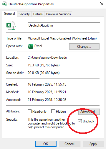
The lesson makes use of several spreadsheet tools, BV Sheet 3 Qubits Task 1.xlsm (etc.), which use embedded macros. Your security settings may block the macros when the file is downloaded. In order to enable them again, you should right click on the file, click “Properties”, and then “Unblock”, as shown below:
Introduction
Imagine you’re in an arcade, and you’ve discovered a mysterious slot machine. Here’s how it works: you have three coins – some dimes and some quarters. The machine allows you to throw in these coins in various combinations, and it will either give you nothing or exactly $1. Your goal is to figure out the exact hidden combination of dimes and quarters that unlocks the dollar jackpot.
This arcade game is a playful analogy for the Bernstein-Vazirani algorithm, which solves a similar type of puzzle – but with quantum superpowers! Just as the slot machine has a hidden rule based on your coin choices, this algorithm is all about discovering a secret pattern (a hidden string of 0s and 1s) that determines the output of a special function. The challenge? Doing it as efficiently as possible.
How to play (students and teacher)
- Students have three coins to start with, represented as bits (0 for dimes and 1 for quarters).
- The slot machine (teacher) has the key (hidden string) and evaluates the input combination and gives the result: 0 (no dollar) or 1 (jackpot!).
- Students’ mission is to guess the exact rule (the hidden string) that determines the result.
Mathematical formulation of the problem
Imagine we have a mystery box represented by a function . This box is special because when you give a binary number with bits, it returns either or . The function is defined using a fixed secret binary number , where each is either or .
To compute , the function follows these steps:
- Take an -bit input , where each is either or .
- Multiply each input bit by the corresponding bit in : .
- Check the result of the sum:
- If the sum is even, the function outputs .
- If the sum is odd, the function outputs .
Task 1
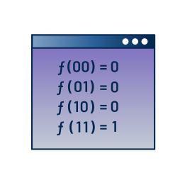
Use the hidden binary number for the case and complete the following table by computing .
| Input x |
| Odd | Even | Output |
|---|---|---|---|---|
|
| x | 0 | |
|
| x | 1 | |
| ||||
| ||||
| ||||
| ||||
| ||||
|
Analyse the Results: How many and which combinations of quarters and dimes will result in a 1$ win. Notice how the outputs depend on the hidden pattern. This pattern is the key to understanding the function’s behaviour.
|
|
|
|
|---|---|---|---|
| 0 | 0 | 0 | 0 |
| 0 | 0 | 1 | 1 |
| 0 | 1 | 0 | 0 |
| 0 | 1 | 1 | 1 |
| 1 | 0 | 0 | 1 |
| 1 | 0 | 1 | 0 |
| 1 | 1 | 0 | 1 |
| 1 | 1 | 1 | 0 |
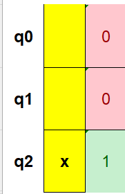
Task 1.xlsm shows the first problem. The blue cells in column E show the inputs to the function, the green cells in column J show the coefficients corresponding to the hidden string, and the red cell in column AC shows the output of the function.
The tool may be used to demonstrate the effect of setting the values as shown in the first two rows of the table in Exercise 1.
Task 2
Now we focus on the actual problem to find the hidden string of a function from the table below:
|
|
|
|
|---|---|---|---|
| 0 | 0 | 0 | 0 |
| 0 | 0 | 1 | 1 |
| 0 | 1 | 0 | 0 |
| 0 | 1 | 1 | 1 |
| 1 | 0 | 0 | 1 |
| 1 | 0 | 1 | 0 |
| 1 | 1 | 0 | 1 |
| 1 | 1 | 1 | 0 |
Find the most efficient strategy to determine the string :
- How many queries do we need?
- Which input values would you use to determine the string most efficiently?
- What is the hidden string?
Quantum computer simulation with the IBM Composer
1. In this first approach, we use a classical algorithm to find the hidden string.
Open https://quantum.ibm.com/composer/files/new . The circuit below implements a particular string, which we are trying to figure out.
Example: Input .
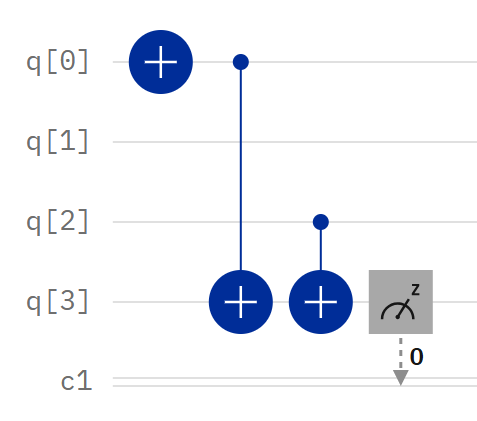
- The input values are the inputs from the first three qubits .
- The function value is the output from .
- All qubits are initialized to input value . In order to change the input value from to , apply to the respective qubit.
- Measurement
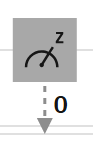 of the last qubit gives .
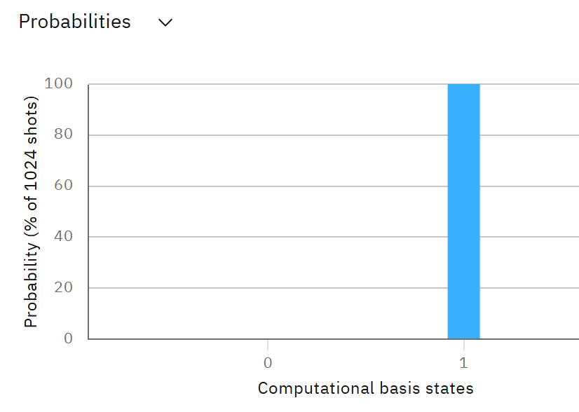
The measured value, in this case , is the function value , which can be read from the graph that shows the simulation of the measurement probability.
We need 3 queries.
Use the combinations , , since
Result:
Task 2.xlsm shows the second problem, with the coefficients hidden. It can be used before the second exercise to encourage students to think about their strategy for finding the hidden coefficients.
Students can suggest input values for the , observe the effect on the output, and then attempt to guess the hidden values. The coefficients can also be changed to different combinations if you do not wish to use the same values as in the exercise.
Task 3
Build the above quantum circuit and use the quantum composer to complete the table below:
| 0,0,0 | 1,0,0 | 0,1,0 | 0,0,1 | 1,1,0 | 1,0,1 | 0,1,1 | 1,1,1 |
| 1 |
2. In this second approach we use the Bernstein Vazirani quantum algorithm to find the hidden string.
The quantum algorithm uses the circuit below. The function is, as before, implemented by the 2 CNOT gates. The hidden output string is obtained after measuring the output of the first 3 qubits. Similar as in the case of the Deutsch Algorithm, the initial Hadamard gates create a superposition of all possible input states.
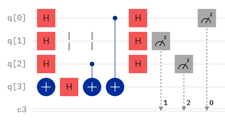
Build the Quantum algorithm and confirm that the simulation indeed reveals the string you found classically in problem 3.
Notice: It took 3 queries classically, but only one query using the quantum algorithm.
In order to explore how the quantum algorithm solves the problem, let’s look at the two dimensional example, , which state evolution we can easily track with help from an Excel sheet.
Download the Excel sheet.
Task 3.xlsm shows the circuitry that students will implement in the IBM Composer. It can be used to demonstrate the effect that students should observe when changing the states of the input qubits in the Composer.
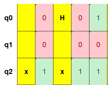
Task 3.2.xlsm shows the circuitry for finding the hidden string with a single query, using Hadamard gates before and after the function. It is configured for the problem in the sheet, but can be reconfigured for other hidden strings by changing the coefficients and redrawing the circuit diagram.
Rows 17–20 of the “BV Game” sheet perform the tensor products and matrix multiplications corresponding to the Hadamard and CNOT gates. These rows may be expanded if the teacher wishes to discuss the detailed effect of the gates on the qubit states.
Task 4
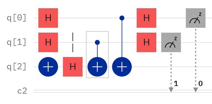
Build the circuit below one gate at a time as you fill in the Excel sheet one gate at a time. Confirm that your Excel agrees with the state evolution from the composer.
Some help how to get started. Use ket notation, explain that I drop the normalisation in the Excel.
Initially all qubits are in state :
The -Gate is acting on and flips the total state to , which we note in our table:
The Hadamard gate acting on and creates a superposition . The total state is therefore
For simplicity, we drop the normalisation factor and denote the final state in our table as
Finish the Excel table and answer the following questions:
- What do the two Hadamard gates in the beginning accomplish?
- Why is there an -Gate at the beginning of the output qubit? Look what would happen if the -Gate was missing.
- What is the purpose of the last two Hadamard gates?
- What string does the measurement reveal?
All images are screenshots taken from Composer | IBM Quantum Platform.
Share this page