Deutsch’s algorithm - Computational approach

Overview
Overview
Keywords: algorithm, superposition
Age group: 16-18 years
Required knowledge/skills: none
Time frame: 40 minutes
Author: Sam Robbins (UK)
Learning objectives
The aim of the lesson is to learn about the Deutsch algorithm for discovery of a mystery function. It shows how classical approaches to the problem are unable to discover the hidden function in fewer than two queries, but that a quantum approach can find the class of functions in one. The lesson introduces the idea of using superposition to probe multiple different states at once, which is the key principle behind all of the later algorithms in this course.
Lesson plan
| Timing in minutes | Lesson phases | Activity | Material |
|---|---|---|---|
| 0–10 | Exercise 1 | Students experiment with spreadsheet and write down strategy for deducing hidden function. | Worksheet & Spreadsheet tool |
| 10-20 | Exercise 2 | Students experiment with spreadsheet and write down strategy for deducing class of hidden functions. | Worksheet & Spreadsheet tool |
| 20-30 | Exercise 3 | Students use spreadsheet to deduce which circuit corresponds to which function. | Worksheet & Spreadsheet tool |
| 30-40 | Exercise 4 | Students use spreadsheet/quantum composer[1] to find the strategy behind the Deutsch Algorithm. | Worksheet & Spreadsheet tool/Quantum Composer |
You can download the worksheet (as pdf and docx) and the spreadsheet (as excel) at the end of the page.
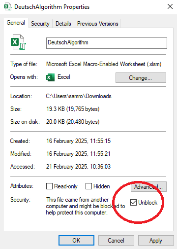
The lesson makes use of a spreadsheet tool called DeutschAlgorithm.xlsm which uses embedded macros. Your security settings may block the macros when the file is downloaded. In order to enable them again, you should right click on the file, click “Properties”, and then “Unblock”, as shown below:
Conceptual introduction
Deutsch's algorithm, developed by David Deutsch in 1985, marks a significant milestone in the world of computing. It is the first instance where a quantum algorithm showed a potential advantage over classical algorithms. This discovery opened the door to the idea that computers based on the principles of quantum mechanics could solve certain types of problems more efficiently than traditional computers. Deutsch's work laid the foundation for quantum computing, inspiring further research and development in this exciting field. In this lesson, you will learn how Deutsch's algorithm works. To fully grasp its significance, you will first need to understand how the problem the algorithm solves can be approached using classical computing methods.
Student exercises and teacher notes
The problem
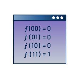
Imagine we have a black box function which takes an input of a single classical bit of data (0 or 1) and returns an output of another single classical bit of data (0 or 1). There are four possible functions this could be:
| f1(0)=0 f1(1)=0 | f2(0)=1 f2(1)=1 | f3(0)=0 f3(1)=1 | f4(0)=1 f4(1)=0 |
The problem is we do not know which function is inside the black box. Our task is to work out which it is just by changing the inputs to the black box and viewing the outputs.
Exercise 1
The “Deutsch Functions” spreadsheet shows how these four functions operate and has a mystery function generator. Click on the “Generate mystery function” button to pick one of the four functions at random. If you change the input in Cell B12 the output of the mystery function will be returned in Cell E12. How can you deduce what the mystery function is by altering the inputs and how many guesses does it take? Justify your answer.
The students should work out that it is impossible to find the function in fewer than two guesses. Note that the students may check their guesses each time by pressing the “Reveal Function” button.
Constant functions versus balanced functions
Suppose now we group the four possible functions into two classes as follows:
| Constant functions | Balanced functions | ||
| f1(0)=0 f1(1)=0 | f2(0)=1 f2(1)=1 | f3(0)=0 f3(1)=1 | f4(0)=1 f4(1)=0 |
Exercise 2
Using the spreadsheet again, how many guesses does it take to establish whether the mystery function is either a constant function or a balanced function? How does this compare to finding the actual function itself? Justify your answer.
The answer (again) is that it is impossible to find the function in fewer than two guesses.
Summary of classical results
We have seen that for both of these problems it takes two queries to find the desired result using classical search techniques. For the first case (finding the specific function), a quantum computer would also require two queries. However, for the second case (deciding whether the function is constant or balanced), quantum computing can provide a radical improvement.
Building the function on a quantum computer
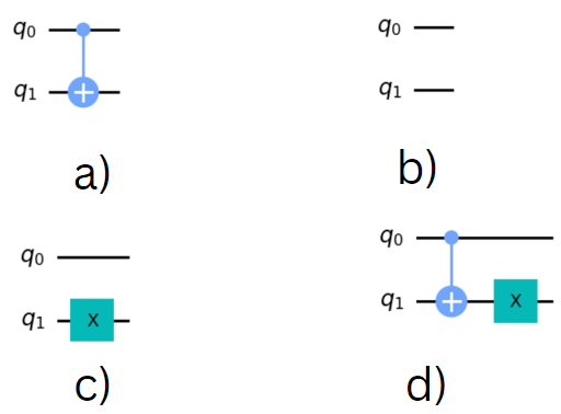
The first step to investigating the problem on a quantum computer is to construct the functions using quantum gates. It is possible to construct all of the four functions using combinations of NOT gates, CNOT gates and no gates at all.
We will need two qubits: q0 which will take the input of the function and q1 which will return the output (after being initial set to state ).
Use the IBM quantum composer to build each of the following four circuits:
Example
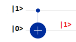
For circuit (a), if we set the input qubit q0 to state and the output qubit q1 initially to state , we see that the final state of q1 is also state (as the CNOT gate is not triggered):
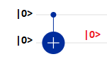
This means that an input of 0 for the function is mapped to an output of 0.
If we now change the input qubit q0 to state , we see that the final state of is now state (as the CNOT gate is now triggered, flipping the state of q1):
This means that an input of 1 for the function is mapped to an output of 1.
These mappings correspond to function f3 (the first of the balanced functions)
Exercise 3
The spreadsheet “Quantum Circuits” contains each of the four circuits shown. The input state for q0 is shown in the bold blue cells, the final state for the output qubit q1 is shown in the bold red cells. By changing the initial inputs to q0 and measuring the final outputs of q1, work out which function (f1, f2, f3 and f4) each of the circuits (b), (c) and (d) corresponds to. Write your answers below:
a) f3 ; b) f1 ; c) f2 ; d) f4
Finding the mystery function using a quantum computer
The technique we will use here employs superposition through the application of Hadamard gates. This is one of the most important tricks of quantum computing and we will see it used in every quantum search algorithm in this course!
Create the following circuit in the IBM quantum composer:
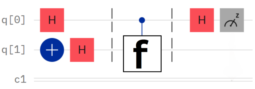
Note that the NOT gate is used to initialise the state of q1 to which the absence of a NOT gate on q0 means this qubit is initialized to state .
Exercise 4
This exercise can be done either using a quantum composer or using the spreadsheet “Quantum Circuits with Hadamards”. Initialise q0 to state and q1 to , then insert each of the circuits for f1, f2, f3 and f4 and in the section of the circuit marked with the mystery function box f. Look at the values that takes after measurement. How can this information be used to deduce whether a function is balanced or constant? How many queries does it now take to show this? Write your answers below:
The final state of the input qubit is for both of the constant functions and for both of the balanced functions. This has allowed us to determine which of the two classes the mystery function belongs to in one query.
The key learning points that students will see again as the course progresses are:
- (1) Hadamards (by creating a superposition state) allowed us to find information about multiple inputs at once.
- (2) Information was gained by looking at the final state of the input qubits.
Summary of quantum results
By using superposition, we were able to find whether the function was constant or balanced in one query rather than two, i.e. a quantum computer can solve this problem twice as fast as a classical computer. There are two important points the Deutsch problem also highlights:
- Quantum computers cannot outperform classical computers in every situation. As we have seen here, the quantum algorithm only helped us with the problem of constant versus balanced functions, not which specific function was in the black box. Whether a problem can be solved by a quantum computer always requires careful thought.
- The solution to this problem was found by looking at the input qubit rather than the output qubit. Information was gained in the input qubit at the expense of information lost in the output qubit. Quantum computing often involves such trade-offs, and we often have to look for solutions in unusual places!
While Deutsch’s problem is a slightly artificial example, it showed the potential for quantum computers and paved the way for more meaningful quantum algorithms that we will explore in the next lessons.
Teaching Materials
Deutsch Algorithm Worksheet PDF
Download FileDeutsch Algorithm Worksheet docx
Download FileDeutsch Algorithm: Worksheet & Spreadsheet (Excel)
Download FileShare this page