Qubits, Quantum Gates and Quantum Circuits – a Computer Science Perspective: Part 2 Quantum Gates and Quantum Circuits
Context
This material is part of the three‑part unit Qubits, Quantum Gates and Quantum Circuits – a Computer Science Perspective. Part 2 introduces students to quantum gates and quantum circuits, explaining their purpose and how they manipulate the state of a qubit.
1. Quantum gates and quantum circuits
Exercises for students
Exercise 1: Define the classical logic gates “AND”, “OR”, “XOR” and “NOT”. List the corresponding truth tables. Research the results of “NOT (A AND B)” or “NOT (A OR B)”.
For exercise 1
Truth table of the logic gate “AND”:
| A | B | A AND B |
|---|---|---|
| False | False | False |
| False | True | False |
| True | False | False |
| True | True | True |
Truth table of the logic gate “OR”:
| A | B | A OR B |
|---|---|---|
| False | False | False |
| False | True | True |
| True | False | True |
| True | True | True |
Truth table of the logic gate “XOR”:
| A | B | A XOR B |
|---|---|---|
| False | False | False |
| False | True | True |
| True | False | True |
| True | True | False |
Truth table of the logic gate “NOT”:
| A | NOT A |
|---|---|
| False | True |
| True | False |
“NOT (A AND B)” is equivalent to “(NOT A) OR (NOT B)”:
| A | B | A AND B | NOT (A AND B) |
|---|---|---|---|
| False | False | False | True |
| False | True | False | True |
| True | False | False | True |
| True | True | True | False |
| A | B | NOT A | NOT B | (NOT A) OR (NOT B) |
|---|---|---|---|---|
| False | False | True | True | True |
| False | True | True | False | True |
| True | False | False | True | True |
| True | True | False | False | False |
“NOT (A OR B)” is equivalent to “(NOT A) AND (NOT B)”:
| A | B | A OR B | NOT (A OR B) |
|---|---|---|---|
| False | False | False | True |
| False | True | True | False |
| True | False | True | False |
| True | True | True | False |
| A | B | NOT A | NOT B | (NOT A) AND (NOT B) |
|---|---|---|---|---|
| False | False | True | True | True |
| False | True | True | False | False |
| True | False | False | True | False |
| True | True | False | False | False |
These two equations are called de Morgan’s laws.
Exercise 2: Compare handling the logic gates “AND” and “OR” with the multiplication and addition of numbers.
(Classical logic gates are covered in the lesson Classical Computing – Introduction to Logic Gates)
For exercise 2
The logic gate "AND" can be compared to multiplication: if "False" is identified with 0 and "True" with 1. If 2 is also identified as “True”, the logic gate "OR" corresponds to addition. If, on the other hand, only the last bit of the addition is considered (i.e. 2 is identified as "False"), the "XOR" logic gate corresponds to addition. With this assumption (2 is identified as “False”), "NOT" corresponds to adding 1.
Definitions
Just as classical gates are used in classical computers to perform elementary operations on classical bits, quantum gates are used in quantum computers to manipulate qubits.
To run a programme on a quantum computer, the appropriate elementary quantum gates are selected and applied to one or more qubits. This can be illustrated in a quantum circuit that shows how the various components of the programme – qubits and gates – are assembled.
Definition of a quantum gate
In quantum computers, operations are performed using quantum gates. Quantum gates act on one or more qubits and can be represented by a unitary matrix. When qubits are manipulated using quantum gates, this corresponds to physical changes in these qubits. Examples: The qubit flips from one basis state to another, or it is brought into a superposition of the basis states.
Definition of a quantum circuit
A quantum circuit is a visual representation of a quantum algorithm: it can be used to represent computing code for a quantum computer. A quantum circuit consists of qubits as well as of quantum gates that are applied to these qubits. In a quantum circuit, time flows from left to right. At the beginning – on the left – are the qubits. The quantum gates are then applied one after the other, from left to right, to the qubits. Measurements and their results are also represented in a quantum circuit. They are usually located on the far right, or sometimes in between.
Assembling a quantum circuit
Quantum circuits are very useful when it comes to programming a quantum computer. The steps are:
- Prepare one or several qubit(s) in an initial state (e. g. ).
- Apply one or several quantum gates on the qubit(s).
- Perform a measurement and obtain a result.
One can assemble a quantum circuit visually using a graphical interface or by using a programming language, like for instance Qiskit.
A quantum circuit is usually run many times because quantum computers are susceptible to noise: even if the probability of measuring a certain result is 100% "0", the result is sometimes not "0" – due to noise. Therefore, quantum circuits are usually run a number of times called “shots” (for instance 1000 shots). The larger the number of shots, the clearer the "correct" result stands out – for example, that 1 + 1 indeed equals 2.
Quantum circuits can be programmed by simply dragging and dropping the corresponding quantum gates in a designated field.
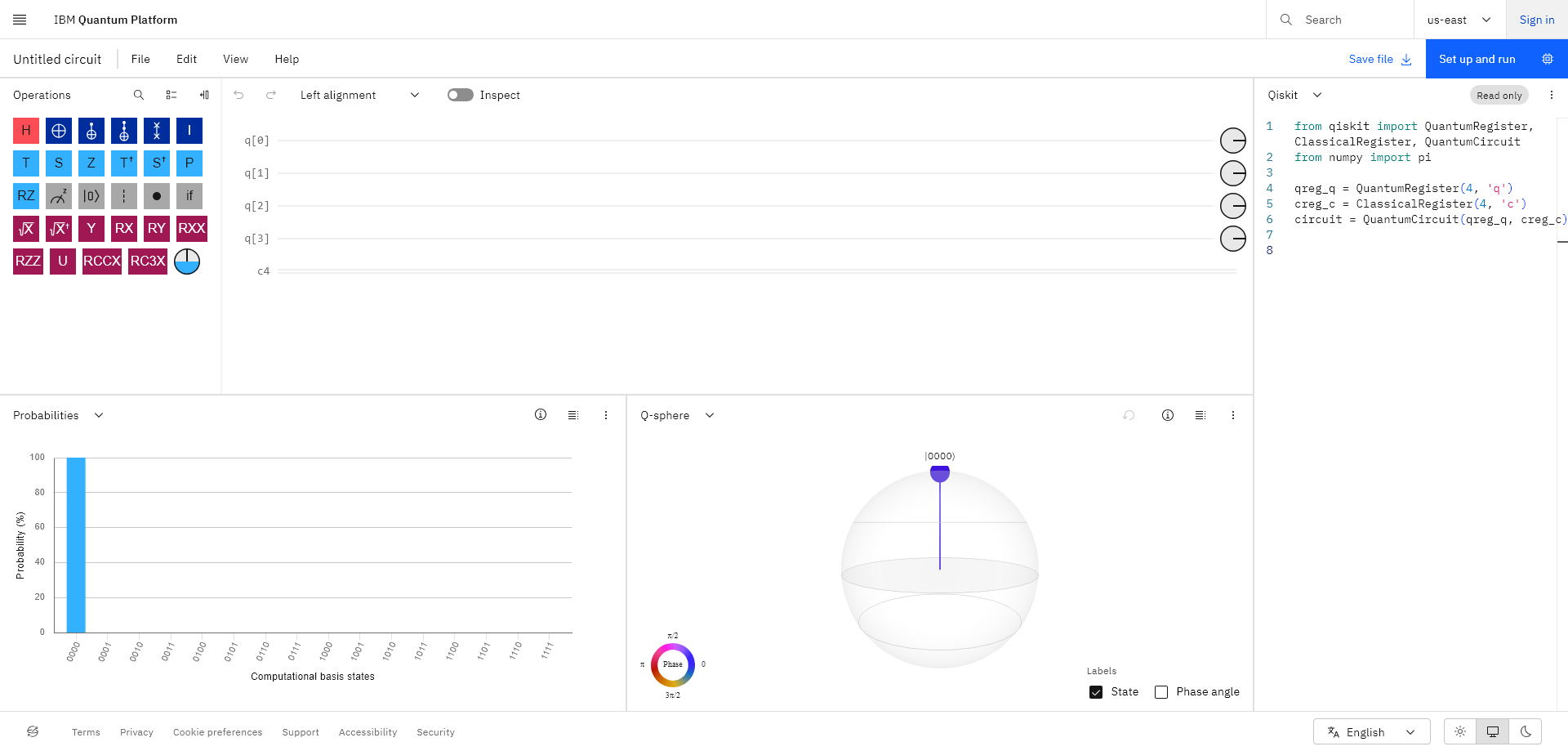
In the case of the IBM Quantum Composer, operations are dragged from a set of operations at the top left into the field in the middle of the screen. The number of qubits and the number of classical bits for the quantum circuit can be set under <Edit>–<Manage Registers>. The probability and the state of the system are predicted at the bottom of the screen, and export options – for example to Qiskit – are offered on the right. Without an account, you can use the built-in simulator, which runs the circuit on a classical computer and shows what would happen in an ideal, noise-free quantum system.
You find additional information including how to access real quantum hardware in this introduction to Qiskit here Programming quantum circuits.
Example: Flipping the state of a qubit using the Pauli-X gate
The Pauli-X gate changes the state of a qubit from to , or from to : it flips the state of a qubit. Because of its similarity with the NOT operation on classical bits, it is also called a NOT (quantum) gate.
The Pauli-X gate can be represented by the matrix :
and
.
This is described in concrete terms and step by step below using the above example (a Pauli-X gate is applied to a qubit in the state ).
The quantum circuit of a Pauli-X gate applied to a qubit looks like this:
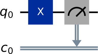
Fig. 1: In this quantum circuit, a Pauli-X gate is applied to a qubit and a measurement is performed.
In Figure 1, is the quantum register – just imagine it as saying, "a qubit is prepared in a specific initial state so that one or more quantum gates can be applied to it". The “q” in stands for “quantum”, and the “0” means that this is the first (and in this case only) qubit. A second qubit could be prepared in the register , a third qubit in , and so on. The blue square with the “X” symbolises the Pauli-X gate. The grey square (depicting a kind of "measuring device") indicates that a measurement is performed. The arrow indicates that a measurement is performed on the qubit . The measurement yields a real number (either 0 or 1 in this case), so the register in which the result of the mesurement is stored is a classical register labelled (“c” stands for “classical”, and “0” means that it is the first and only register needed in this example).
Using Qiskit
Instead of assembling a programme visually using a quantum circuit, one can also write it using Qiskit, an open source framework developed by IBM for programming quantum computers.
# One quantum register is required.quantum_registers = QuantumRegister(1, 'q')# One classical register is required.classical_registers = ClassicalRegister(1, 'c') # Both registers are added to the quantum circuit.circuit = QuantumCircuit(quantum_registers, classical_registers)# The Pauli-X gate is applied to the quantum register.circuit.x(quantum_registers[0])# A measurement is performed on the quantum register and the result is “delivered” to the classical register.circuit.measure(quantum_registers[0], classical_registers[0])
These lines of code only describe the actual quantum circuit. They must be inserted at the point marked in red in the following code:[1]
# Create a quantum circuitfrom qiskit import QuantumRegister, ClassicalRegister, QuantumCircuit# Optimise the quantum circuitfrom qiskit.transpiler.preset_passmanagers import generate_preset_pass_manager# Access IBM Quantumfrom qiskit_ibm_runtime import QiskitRuntimeService, SamplerV2 as Sampler
service = QiskitRuntimeService(channel="ibm_quantum", token="Insert your API token here, see Profile Settings -> API token")# Choose the least busy quantum computer as backendbackend = service.least_busy(operational=True, simulator=False) # Create a sampler, that will run the job on the chosen backendsampler = Sampler(backend)# Create a pass manager that will optimise the quantum circuit for the chosen backend; optimisation level 3 is the highest possible level. Lower levels are easier to understand but produce less accurateresultspassmanager = generate_preset_pass_manager(3, backend=backend)
# Insert the code for programming your quantum circuit.
# Create the optimised quantum circuitoptimized_circuit = passmanager.run(circuit)
# Add the quantum circuit as a job to the job queuejob = sampler.run([optimized_circuit], shots=1000)# Print the Job IDprint("job id:", job.job_id())# Wait for the results; this can take some time, but the results will also be available on the IBM Quantum platform if the job is interruptedresult = job.result()print(result[0].data.c.get_counts())
The code above includes a so-called transpiler that optimises the quantum circuit. This is necessary because real quantum computers do not always offer all the desired gates. Some optimisations also reduce the quantum circuit’s noise and achieve better results.
The following is the result of the above programme run on a real quantum computer (the y-axis displays the number of shots):
Fig. 2: A Pauli-X quantum gate is applied to a qubit in the state | 0 ⟩ . The result shows that the qubit is now in the other basis state, the state | 1 ⟩ . The higher the number of shots (plotted on the y-axis), the more clearly the "correct" result stands out. The more the noise is suppressed, the smaller the left bar in Fig. 2.
2. Elementary quantum gates
The identity gate
Besides the Pauli-X gate, another elementary and very simple quantum gate is the identity gate. It does not change the state of the qubit.
Its matrix is the identity matrix :
and
.
In combination with other gates, the identity gate – i.e. “do nothing” – can be useful in some cases.
The quantum circuit of an identity gate applied to a qubit looks like this:
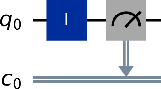
Fig. 3: In this quantum circuit, an identity gate is applied to a qubit. Subsequently, a measurement is performed.
quantum_registers = QuantumRegister(1, 'q')classical_registers = ClassicalRegister(1, 'c')circuit = QuantumCircuit(quantum_registers, classical_registers)# apply the identity gate to the circuitcircuit.id(quantum_registers[0])# measurementcircuit.measure(quantum_registers[0], classical_registers[0])
Fig. 4: Result of applying the identity gate to a qubit in the state . It leaves the qubit unchanged.
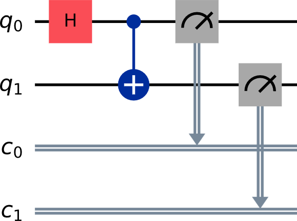
The Hadamard gate
A special gate is the Hadamard gate: starting from the basis state (or the basis state ), it creates a superposition of und , the two basis states of a qubit:
.
The Hadamard gate is represented by the matrix :
and
.
The two amplitudes (i.e. the two coefficients in front of the basis states) in the superposition state are equal, in both cases. The squares of the amplitudes give the probabilities for finding the qubit in state resp. (see Basics of Quantum Physics). This means that the probability for finding the qubit in state is , and the probability for finding the qubit in state is as well.
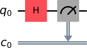
Fig. 5: In this quantum circuit, a Hadamard gate is applied to a qubit. A measurement is then performed.
quantum_registers = QuantumRegister(1, 'q')classical_registers = ClassicalRegister(1, 'c')circuit = QuantumCircuit(quantum_registers, classical_registers)# Apply a Hadamard gate to the qubit in the quantum registry circuit.h(quantum_registers[0])# Measurementcircuit.measure(quantum_registers[0], classical_registers[0])
Fig. 6: A Hadamard gate is applied to a qubit (in state or , in both cases the same result is obtained). In approximately of cases, the qubit is measured in state , and in of cases in state .
Qiskit must be installed in a Python 3 environment: https://docs.quantum.ibm.com/guides/install-qiskit
Share this page