Grover’s Algorithm

Overview
Overview
Keywords: quantum algorithms, search, complexity
Age group: 16-18 years
Required knowledge/skills: quantum states, Hadamard gate, quantum composer
Time frame: 60-90 minutes lesson
Author: Holger Vogts (DE)
Lesson plan
| Timing in minutes | Lesson phases | Activity | Resources |
|---|---|---|---|
| 0–5 | Introduction | Remember linear search from lesson 1. | Worksheet |
| 5–10 | Exercise 1/2 | Find the classical solution (compare with lesson 1) and write the numbers in binary representation. | Worksheet |
| 10–20 | Understanding the oracle gates | The Toffoli gate as oracle is introduced and compared to the CNOT gates used in Bernstein Vazirani. Depending on the student group, this can be done by themselves by reading the chapter or by explanation through the teacher. | Worksheet (page 2 and 3) |
| 20–40 | Exercise 3 | Students do the Grover algorithm in a geometrical approach. They read the chapter “Quantum solution” and transfer the algorithm in task 3 to different numbers. The results should be reviewed before continuing with the next phase. | Worksheet |
| 40–50 | Exercise 4 | Students reflect their solution from the geometrical approach. This is a crucial point in the lesson to understand how Grover’s algorithm works and to compare it to the other algorithms from the previous lessons. | Worksheet |
| 50–60 | Summary | The results from the previous phase are discussed in plenum. The teacher should focus on the comparison to other quantum algorithms as well as to the classical case. | Worksheet |
| 60–end | Exercise 5 | Optional: The algorithm is tested in the quantum composer. The probabilities can be compared with the geometrical approach. | Worksheet, quantum composer |
Student exercises and teacher notes
Imagine you want to crack a safe with a combination lock that has four digits ranging from 0 to 9. You have no clue which numbers might be correct. If you're very lucky, you might hit the right combination on your first try. How many attempts would you need if things go badly? How many attempts would you need on average?
Remember the search in unstructured data in lesson 1 (programming and non-programming versions).
Worksheet
The following tasks are available as worksheet for download as pdf and docx.
The search problem
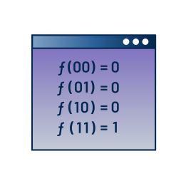
There is a list of N numbers, in which exactly one of the numbers is assigned to 1 (this is the right number) and all other numbers are assigned to 0. The task is to find the position of the number which is assigned to 1 with the least possible number of questions.
The mathematical description of this problem can be done in terms of a function with the following definition. There exists exactly one r from 1 to N with:
Classical solution
Exercise 1: Classical solution
Assuming you don’t know what r is, determine the average number of guesses of x you will input into the function f to find r. What is your strategy for doing this?
Use linear search (compare to Exercise 1 in lesson 1 – programming and non-programming versions), and O(N) steps.
Exercise 2: Binary representation
We will use the binary representation of the numbers from 1 to N. So and r is represented as a string of 0s and 1s of length n.
Find the binary representation of r = 5 in the case N = 16.
The solution is: r = 0101
Implementing the search function using quantum gates
In order to implement the search function, we need to introduce a new gate, known as the Toffoli gate. This is very similar to a CNOT gate, but acts on multiple input qubits. For example:
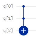
This Toffoli gate will perform a NOT operation on the output qubit q[2] only when both input qubits, q[0] and q[1], are in state . With the output qubit initially set to state , this structure has the same effect as the equivalent to the AND operation in classical computing.
The following table shows the final state of the output qubit, q[2], for all combinations of the two input qubits:
| q[0] |
|
|
|
|
| q[1] |
|
|
|
|
| q [2] (final) |
|
|
|
|
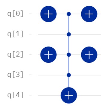
To build the hidden function for the Grover search, we use a combination of an n-input Toffoli gate and single qubit NOT gates.
For our implementation of the Grover Algorithm, we will use a 4-qubit implementation where we are searching for the hidden string 0101. To build the circuit for this, we need a 4-qubit Toffoli gate and NOT gates for the qubits that correspond to 0s in the hidden string. The NOT gates flip these two inputs to so that the Toffoli gate flips the state of the output qubit to only when all of the input states match the hidden string. After the Toffoli gate the corresponding states have to flipped back by NOT gates.
Gate structure for hidden string 0101
The difference between Grover and Bernstein-Vazirani
In the previous lesson, we saw how the Bernstein-Vazirani hidden function could be found in a single step. However, the Bernstein-Vazirani function had the property that it could be constructed using only CNOT gates, and this was the reason why the application of Hadamards led immediately to the discovery of the hidden function.
The objective of Grover is to solve the more realistic problem of identifying whether a particular data item exists within an unstructured set of data. The requirement to use Toffoli gates to do this means that the Bernstein-Vazirani approach does not give us the desired result. However, as in both Deutsch and Bernstein-Vazirani, we begin by putting all input qubits into state , the output qubit into state , and applying Hadamards to all qubits:
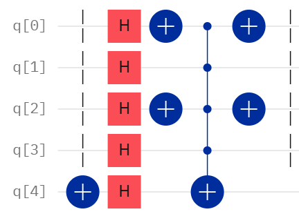
The following table shows the effect on the input qubits happens of this structure:
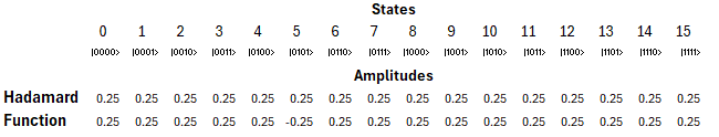
The application of the Hadamards creates a superposition of 16 different states (all the binary combinations of 0s and 1s from 0 to 15). Note that the probability of being in any of a measurement resulting in any particular state is 1/16 and the initial amplitude of each is 1/4. This is the same starting point as in all of our previous algorithms.
However, the application of the hidden function then has a curious effect. All of the amplitudes of the incorrect guesses remain the same, but the coefficient of the correct combination is flipped to have a negative sign.
It is important to understand that this alone will not allow us to find the hidden string. The probability of being in each state is the square of the amplitude, so this state still has the same probability as all others and measurement at this stage would not give us any better chance of finding the hidden string.
However, if we apply further operations to this superposition state, we are able to amplify the magnitude of the state of the hidden string (whilst shrinking all of the others). The following part shows how Grover’s Algorithm does this.
Grover‘s Algorithm: Quantum Solution
Grover’s algorithm tackles our problem using only number of questions, thanks to the power of quantum computing. The algorithm is implemented in the following steps, which we will understand in a geometric picture:
Step I:
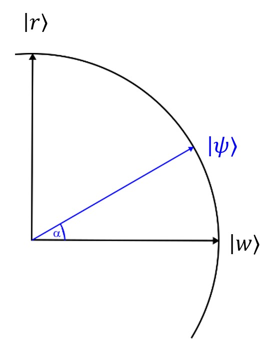
Prepare qubits in state and apply a Hadamard gate to all of them. This gives a superposition of all possible states on the qubits.
This state can be described in a composition of the desired (right) state and the (normalized) sum of all other (wrong) states , which are perpendicular to .
Example:
In the case of we will get
.
If we assume that the desired number is , this can be written as
with
.
The angle can be calculated by the arcsine of the factor of the desired state:
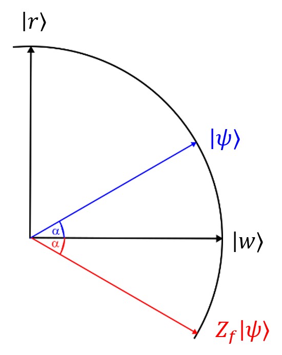
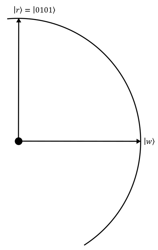
Step II:
Apply the oracle gate to . This gate does exactly one query on the function .
As defined in the previous section, it adds a minus to the state and does not change any other state, which means that the vector is reflected at the vector .
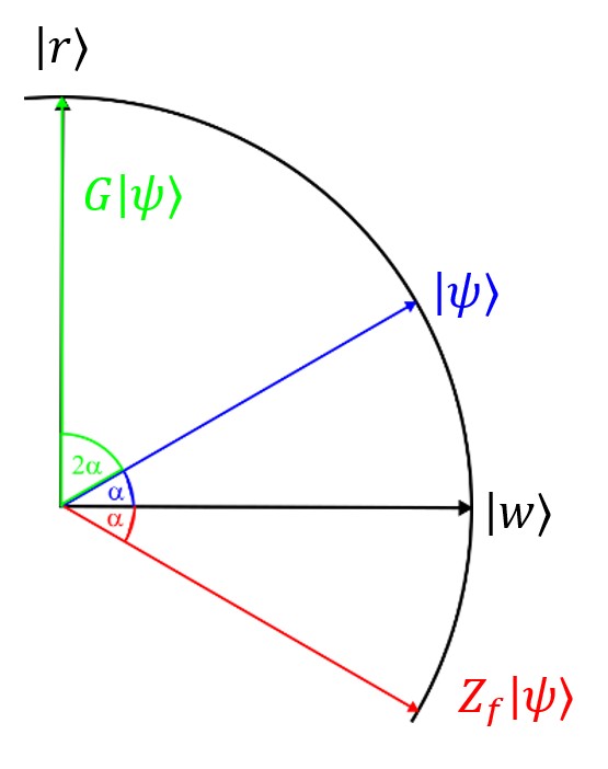
Step III:
Apply a combination of gates, which lead to a reflection of the vector at the vector .
The combination of step II and step III is called Grover operation . This means that the resulting vector is rotated by in direction of the desired state in comparison to the initial state .
In the example N = 4 we have reached the desired state exactly with one step of the Grover operation. In general, the Grover operation has to be repeated as in the next step.
Step IV:
Repeat the Grover operation (step II and step III) subsequently times (so the number of queries on is ) until the state vector is at most parallel to and do a measurement on all qubits.
Exercise 3: Understanding Grover’s Algorithm step by step
Now, you will delve into each step of the algorithm and get an understanding of how often the Grover operation must be repeated.
In this case we set and .
Step I:
Applying the Hadamard operation on all four qubits of the state gives
.
Let us assume that . So
,
whereby is some normalization value.
Calculate the angle from the factor
and draw the corresponding vector in the picture.
Step II: Draw the state vector by reflection of at .
Step III: Draw the state vector by reflection of at .
Step IV: Repeat step II and step III (so ).
The angle can be calculated by
.
After one Grover operation the angle is approximately 44,5°; after the next Grover operation 72,5°.
Exercise 4: Reflecting on your solution
a. Do you think that two repetitions of the Grover operation are sufficient? What would happen if you did more repetitions?
After two repetitions the state is not exactly the desired state, but it has already a large amplitude in the correct direction. Doing a further repetition would change the angle to approximately 101,5°, so the state would correspond a little bit better to the desired state. Doing more repetitions would make the result worse, since the state would remove from the desires direction.
b. The Grover algorithm gives the right answer with high probability and not necessarily exact. Explain this with your solution.
An exact answer of the search problem would require that the quantum state is exactly the desired state. In the case of n=4 this is not possible due to the angles which occur with these numbers. But after two or three Grover operations the probability of getting the right answer in the measurement is much larger than getting the wrong answer since the amplitude is much higher in the right direction rather than in the wrong direction (see conclusions in the worksheet how to handle this problem).
c. How does the angle α behave if n increases? What does this mean for the number of repetitions?
The angle will become smaller if n increases. This means that the Grover operation must be repeated more often to get closer to the desired direction.
(In addition: This will also mean that you will get closer to the desired direction since you can manage the number of repetitions such that you are not more than α away from the desired direction.)
Conclusions
Why does Grover only need steps?
In general, the angle is equal to
which is approximately equal to .
After one Grover operation the current angle is , after the second Grover operation the angle is . For Grover operations the angle is .
To get the right state with a high probability this angle should be close to .
So with
we get ,
which is the optimal number of iterations in the Grover algorithm.
How can I be sure to get the right answer?
The Grover algorithm will in most cases give the result with a high probability and not necessarily exact. To be sure, to get the right answer, it is easy to check the result just by putting the result in the oracle. If the result is not correct, you can just run the Grover operation a second time to get another result to check.
Exercise 5
The circuit shows the 4bit Gover operation with the desired state .
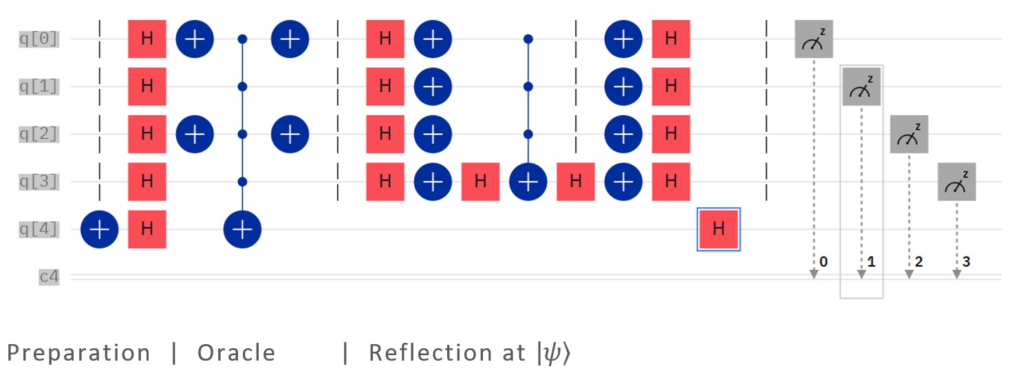
- Implement this circuit in the composer.
- The circuit just implements one Grover operation. Repeat this step in the circuit and compare with your results from task 2.
For a repetition of the Grover operation the oracle and the reflection at must be repeated:
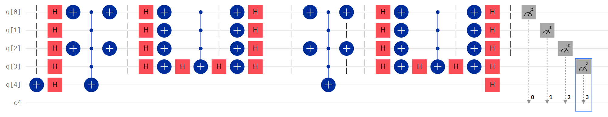
This will result in a probability of the desired state of approximately 90,2 %:
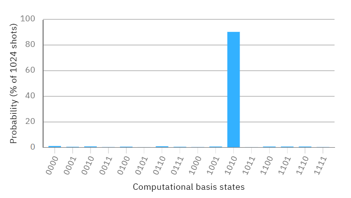
Doing a third repetition will result in a probability of 95,8%.
Share this page