Introduction to search algorithms: Non-programming version
Overview
Overview
Keywords: algorithm, order of complexity, big O notation, linear search, binary search, trial division, cryptography
Age group: 16-18 years
Required knowledge/skills: none
Time frame: 60 min (one lesson)
Author: Sam Robbins (UK)
Lesson plan
| Timing in minutes | Lesson phases | Activity | Resources |
|---|---|---|---|
| 0–10 | Exercise 1 | Students make cards and play a game to work out how long it takes to find data in an unstructured data set. | Worksheet |
| 10–25 | Exercise 2a | Students reuse cards from Exercise 1 to play a game to work out how long it takes to find data in an ordered data set. | Worksheet |
| 25–40 | Exercise 2b | Students cut out the picture cards to play a game to work out how long it takes to find data in an ordered data set. | Worksheet |
| 40–60 | Exercise 3 | Students calculate prime factors of numbers shown and articulate the method used to do so. | Worksheet |
Student exercises and teacher notes
This series of lessons considers the issue of how computers search for data. Search algorithms are some of the most important tools used in computing. In the world of classical computing, there are a number of well-known algorithms for performing searches. For many years, it was thought that the efficiency of these algorithms formed a hard limit on how quickly computers could search for data. The advent of quantum computers promises to change all of this, with new quantum algorithms offering the potential for radical speed-up in a number of areas.
This lesson will cover the basics of three types of three classical algorithm that are used to search for data. In the remainder of the course, we will revisit these algorithms to see how quantum computers can be used to improve upon the performance in each case.
Worksheet
The following tasks are available as worksheet for download as pdf and docx.
Problem 1: Searches in unstructured data arrays
Imagine we have a list of eight names, but the list is not in order. You want to find where one particular name occurs in this list. Here is the list of names:
| Adriano | Birte | Edouard | Elena | Florian | Inez | Niamh | Oliver |
Unfortunately, a computer is not able to scan the whole array at the same time, it can only look at one element of the array at a time and tell you whether the entry for that element matches the one you are looking for or not.
Exercise 1
Make eight cards with the names from above on them. Place them face down on the desk and shuffle them to ensure they are in a random order. Search for the name “Elena” in the cards. What is your strategy for finding the card? Play the game three times. What is the maximum number of guesses it takes you and what is the average number?
The strategy you probably followed was to start with the first element and test each in turn until you found the data item you were looking for. You might also have chosen elements at random (ensuring that you never picked the same one twice), but in fact this would be no better. In either case, the maximum number of guesses you would need was 8 and the (long-run) average number of guesses was 4.5.
The strategy of testing each element in an array until you find a match is known as linear search. In the worst-case scenario, the number of comparisons we need is the same as the size of the data array we are searching. We say that the order of complexity of the algorithm is O(n) (using big O notation), because the number of comparisons we have to perform on an array of n elements is of the order of n.
In classical computing there is no way of searching an unsorted array of data faster than this. However, using a quantum computer, we may be able to perform such a search in O(√n) operations, meaning we can search an array with n elements by a number of comparisons of the order of √n. We will learn about this method, known as Grover’s Algorithm, in Lesson 4.
Once the game is complete, students should explain their strategies. The teacher should then run through linear search (i.e. selecting each data item in turn until the search item is found or every item of data has been checked) and explain that this is the best classical algorithm for searching unsorted data. Linear search has complexity O(n), but the equivalent quantum approach (Grover’s Algorithm, which will be covered in Lesson 4) has complexity O(√n).
Problem 2: Searches in structured data arrays
Exercise 2a: searching an ordered array
Make eight cards with the names on from Problem 1. Place them face down on the desk in alphabetical order. Search for the name “Inez” in the cards. What is your strategy for finding the card? Play the game with each of the different names. What is the maximum number of guesses it takes you and what is the average number?
The best strategy here is to guess in the middle of the array. If you find a match, stop. If your name is higher in the alphabet than the element you checked, go to the mid-point of the upper half of the array and test again. If it is lower, go to the mid-point of the lower half of the array and test again. Keep doing this until you find the name.
Depending on how you chose to round your mid-points, you should have found “Inez” in either two or three guesses. The greatest number of guesses required is four and the average required over all the names (using the algorithm shown) is 2.625.
This algorithm is known as binary search. Knowledge of the structure of the array makes this algorithm much faster than a linear search. In the worst-case scenario, the number of comparisons we need is linked to the logarithm (in base 2) of the number of elements of the array. In the example above, there are 8 elements: log28 = 3. We say that the order of complexity of the algorithm is O(log(n)) (using big O notation), because the number of comparisons we have to perform on an array of n elements is of the order of log(n).
Once game is complete, students should explain their strategies. Teacher should then run through binary search (i.e. always choosing the middle item of the search array and then repeating with the lower or upper half of the array, depending on the comparison made) and explain that this is the best classical algorithm for searching sorted data. Binary search has complexity O(log(n)).
Exercise 2b: searching an array of elements with sets of characteristics
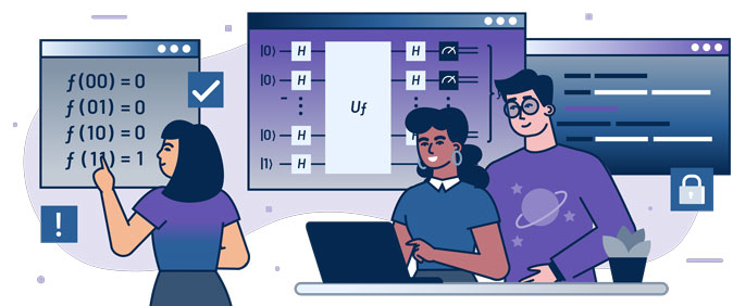
Imagine our characters now have the following facial characteristics:

The game is now to identify one character from the set by asking questions about their appearance. Each question, however, can only be answered “yes” or “no”.
This is a variant of the game “Guess Who”. Cut out the eight pictures shown. One player then picks one at random and the other player has to guess who it is by asking questions. What questions do you ask? How many goes does it take to find the character?
Hopefully, you will have seen that by guessing one of the two possibilities for each characteristic, you could rule out half of the candidates each time. As there were eight characters, it took three questions to uniquely identify the character each time (note that the characters were chosen to represent all unique combinations of the three binary characteristics, so there could be no ambiguity in the final selection).
The answer in all cases is three guesses. This is a variant of the binary search shown in part 2a and, again, the order of complexity of the algorithm is O(log(n)) (though in this case it will take exactly log2n guesses for every search).
In quantum computing, this particular structure of problem has a remarkable solution: the answer can be found using exactly one computation, however large n. It is known as the Bernstein-Vazirani problem, and we shall see how the algorithm works in Lesson 3 (mathematical and computational approach).
Once game is complete, students should explain their strategies. The correct strategy is to guess one characteristic at a time (e.g. “does your character wear glasses?”). This will eliminate half of the characters with each guess, meaning that the correct character can always be found in three guesses. This is a variant of binary search because the search range can again be halved with each iteration. This example has been chosen, because it is equivalent to a particular search problem, known as the Bernstein-Vazirani problem, where the quantum algorithm has O(1) complexity. This algorithm will be covered in Lesson 3 (mathematical and computational approach).
Problem 3: Factoring
Similar techniques to those used in search algorithms are also required for many different mathematical problems, e.g. to find a square root iteratively. One particular problem is how to find the prime factors of a large number.
Exercise 3
Find all the prime factors of the following two numbers: (a) 8192; (b) 6557.
What was your strategy for doing this? How many calculations did it take to find all the prime factors?
One possible algorithm is to test each prime in turn. If the number does not divide by the prime, try the next prime in the list. If it does divide by the prime, calculate the quotient and test whether this number divides by each prime in the list (starting from the beginning again).
This strategy is known as trial division. With a number like 8192, which has many low prime factors, we can break down a number into its prime factors quite quickly (in this case, with 12 calculations). However, where a number has only two similar-sized prime factors, the algorithm is much slower. In the case of 6557 (= 79 × 83), it takes 22 calculations to find the factors. If we were to construct a number which was the product of two primes which were, for example, 600 digits in length, not even a supercomputer would be able to factorise it. The RSA algorithm, which is used worldwide in encryption for the banking system and the wider internet, relies on this key fact for its security. In the classical computing world, this encryption routine is thought to be unbreakable. However, quantum computing may offer a way to break it. In Lessons 5 and 6, you will learn about the RSA encryption system (RSA: the unbreakable code?) and how Shor’s algorithm (Breaking the unbreakable? Shor’s Algorithm) offers a potential method for a quantum computer to it.
Once game is complete, students should explain their strategies. The point of this exercise is to show that factorising numbers by trial division is a computationally slow process, especially where the number is the product of two large primes. The RSA algorithm (on which a large amount of internet encryption is based) relies on the difficulty of factoring large numbers as the basis of its security. Lesson 5 will go through the RSA algorithm (RSA: the unbreakable code?) and Lesson 6 will show how a quantum algorithm (Shor’s algorithm) may one day be able to break it (Breaking the unbreakable? Shor’s Algorithm).
Lesson 2 (which follows this lesson) will explore Deutsch’s algorithm (mathematical and computational approach). The classical approach to this algorithm has not been covered here, as it is an artificial construction with no widely-used application in computing. Its importance, however, is that it was the first example of a problem for which a quantum algorithm was faster than any classical algorithm. The basic elements of the approach used in Deutsch’s Algorithm will inform all the algorithms covered in the later part of this course.
The key to quantum supremacy: superposition
Quantum computing offers a fundamentally different approach to the classical algorithms shown above. The quantum algorithms described in the rest of this course all depend on the use of Hadamard gates to create and unwind superposition states, so before you go further with this course, please check you understand the basics of how quantum gates work.
Superposition gives us a tool for probing all possible input states at once. It will not always be the case that this will provide the search result in one go. In some cases, we may not know the answer with 100% certainty, but the probabilistic advantage we will gain can provide sufficient information to be a massive improvement over the classical world. Quantum computing involves considerable creativity and ingenuity, and in the remainder of this course we will show you some of the remarkable and beautiful tricks that will fundamentally change how we are able to search for data in the future.
The first realisation of the potential for quantum supremacy in search problems was Deutsch’s Algorithm, which was first proposed by David Deutsch in 1985. In Lesson 2 (mathematical and computational approach), we will explore this algorithm, which forms the basis for all the subsequent algorithms in this course.
Share this page