Qubits, Quantum Gates and Quantum Circuits – a Computer Science Perspective: Part 3 The CNOT Gate and Entanglement

Context

This material is part of the three‑part unit Qubits, Quantum Gates and Quantum Circuits – a Computer Science Perspective. Part 3 introduces the CNOT and demonstrates how the gate operates and interacts with previous concepts. A key focus is generating entanglement by using a Hadamard gate followed by a CNOT gate. This final section also includes 12 cumulative exercises that reinforce concepts from all three parts.

You can download a standalone version of the exercises for the students as a docx or PDF.

Content of Part 3

1. The CNOT gate - a gate acting on two qubits
2. Entangling two qubits with a Hadamard and a CNOT gate
3. Exercises

1. The CNOT gate - a gate acting on two qubits

Some gates act on more than one qubit, for example the CNOT gate (also called “controlled NOT gate”). It applies the Pauli-X gate (also called NOT gate) to a qubit if and only if another qubit, the so-called control qubit, is in the state $| 1 ⟩$ .

The matrix representing the CNOT gate is:
$CNOT = [\begin{matrix} 1 & 0 & 0 & 0 \\ 0 & 1 & 0 & 0 \\ 0 & 0 & 0 & 1 \\ 0 & 0 & 1 & 0 \end{matrix}]$ .

Let us assume that the first qubit, the control qubit, is in the state $| 0 ⟩$ , and the second qubit is in the state $| 0 ⟩$ as well. We can represent the combination of these two qubits by $| 00 ⟩$ in bra-ket notation, the corresponding vector being $[\begin{matrix} 1 \\ 0 \\ 0 \\ 0 \end{matrix}]$ (see Part 1: Qubits and their representations).

Calculating the results of a CNOT gate Calculating the results of a CNOT gate

$\begin{matrix} CNOT \cdot | 00 ⟩ = [\begin{matrix} 1 & 0 & 0 & 0 \\ 0 & 1 & 0 & 0 \\ 0 & 0 & 0 & 1 \\ 0 & 0 & 1 & 0 \end{matrix}] \cdot | 00 ⟩ = [\begin{matrix} 1 & 0 & 0 & 0 \\ 0 & 1 & 0 & 0 \\ 0 & 0 & 0 & 1 \\ 0 & 0 & 1 & 0 \end{matrix}] \cdot [\begin{matrix} 1 \\ 0 \\ 0 \\ 0 \end{matrix}] \\ = [\begin{matrix} 1 \cdot 1 + 0 \cdot 0 + 0 \cdot 0 + 0 \cdot 0 \\ 0 \cdot 1 + 1 \cdot 0 + 0 \cdot 0 + 0 \cdot 0 \\ 0 \cdot 1 + 0 \cdot 0 + 0 \cdot 0 + 1 \cdot 0 \\ 0 \cdot 1 + 0 \cdot 0 + 1 \cdot 0 + 0 \cdot 0 \end{matrix}] = [\begin{matrix} 1 \\ 0 \\ 0 \\ 0 \end{matrix}] = | 00 ⟩ \end{matrix}$

$\begin{matrix} CNOT \cdot | 01 ⟩ = [\begin{matrix} 1 & 0 & 0 & 0 \\ 0 & 1 & 0 & 0 \\ 0 & 0 & 0 & 1 \\ 0 & 0 & 1 & 0 \end{matrix}] \cdot | 01 ⟩ = [\begin{matrix} 1 & 0 & 0 & 0 \\ 0 & 1 & 0 & 0 \\ 0 & 0 & 0 & 1 \\ 0 & 0 & 1 & 0 \end{matrix}] \cdot [\begin{matrix} 0 \\ 1 \\ 0 \\ 0 \end{matrix}] \\ = [\begin{matrix} 1 \cdot 0 + 0 \cdot 1 + 0 \cdot 0 + 0 \cdot 0 \\ 0 \cdot 0 + 1 \cdot 1 + 0 \cdot 0 + 0 \cdot 0 \\ 0 \cdot 0 + 0 \cdot 1 + 0 \cdot 0 + 1 \cdot 0 \\ 0 \cdot 0 + 0 \cdot 1 + 1 \cdot 0 + 0 \cdot 0 \end{matrix}] = [\begin{matrix} 0 \\ 1 \\ 0 \\ 0 \end{matrix}] = | 01 ⟩ \end{matrix}$

$\begin{matrix} CNOT \cdot | 10 ⟩ = [\begin{matrix} 1 & 0 & 0 & 0 \\ 0 & 1 & 0 & 0 \\ 0 & 0 & 0 & 1 \\ 0 & 0 & 1 & 0 \end{matrix}] \cdot | 10 ⟩ = [\begin{matrix} 1 & 0 & 0 & 0 \\ 0 & 1 & 0 & 0 \\ 0 & 0 & 0 & 1 \\ 0 & 0 & 1 & 0 \end{matrix}] \cdot [\begin{matrix} 0 \\ 0 \\ 1 \\ 0 \end{matrix}] \\ = [\begin{matrix} 1 \cdot 0 + 0 \cdot 0 + 0 \cdot 1 + 0 \cdot 0 \\ 0 \cdot 0 + 1 \cdot 0 + 0 \cdot 1 + 0 \cdot 0 \\ 0 \cdot 0 + 0 \cdot 0 + 0 \cdot 1 + 1 \cdot 0 \\ 0 \cdot 0 + 0 \cdot 0 + 1 \cdot 1 + 0 \cdot 0 \end{matrix}] = [\begin{matrix} 0 \\ 0 \\ 0 \\ 1 \end{matrix}] = | 11 ⟩ \end{matrix}$

$\begin{matrix} CNOT \cdot | 11 ⟩ = [\begin{matrix} 1 & 0 & 0 & 0 \\ 0 & 1 & 0 & 0 \\ 0 & 0 & 0 & 1 \\ 0 & 0 & 1 & 0 \end{matrix}] \cdot | 11 ⟩ = [\begin{matrix} 1 & 0 & 0 & 0 \\ 0 & 1 & 0 & 0 \\ 0 & 0 & 0 & 1 \\ 0 & 0 & 1 & 0 \end{matrix}] \cdot [\begin{matrix} 0 \\ 0 \\ 0 \\ 1 \end{matrix}] \\ = [\begin{matrix} 1 \cdot 0 + 0 \cdot 0 + 0 \cdot 0 + 0 \cdot 1 \\ 0 \cdot 0 + 1 \cdot 0 + 0 \cdot 0 + 0 \cdot 1 \\ 0 \cdot 0 + 0 \cdot 0 + 0 \cdot 0 + 1 \cdot 1 \\ 0 \cdot 0 + 0 \cdot 0 + 1 \cdot 0 + 0 \cdot 1 \end{matrix}] = [\begin{matrix} 0 \\ 0 \\ 1 \\ 0 \end{matrix}] = | 10 ⟩ \end{matrix}$

Note that the second qubit is “flipped” when the first qubit is in the state $| 1 ⟩$ .

2. Entangling two qubits with a Hadamard and a CNOT gate

The CNOT gate allows to entangle two qubits. The procedure goes as follows:

Take two qubits in the state $| 00 ⟩$ .
Apply a Hadamard gate on the first qubit (See "The Hadamard gate" in Part 2):
$H \cdot | 0 ⟩ = \frac{1}{\sqrt{2}} \cdot [\begin{matrix} 1 & 1 \\ 1 & - 1 \end{matrix}] \cdot | 0 ⟩ = \frac{1}{\sqrt{2}} \cdot | 0 ⟩ + \frac{1}{\sqrt{2}} \cdot | 1 ⟩$ .
The first qubit is in a superposition state, while the second qubit remains in the state $| 0 ⟩$ .
The state of this two-qubit system can thus be written as: $\frac{1}{\sqrt{2}} \cdot | 00 ⟩ + \frac{1}{\sqrt{2}} \cdot | 10 ⟩$ .
Or in vector notation: $\frac{1}{\sqrt{2}} \cdot [\begin{matrix} 1 \\ 0 \\ 0 \\ 0 \end{matrix}] + \frac{1}{\sqrt{2}} \cdot [\begin{matrix} 0 \\ 0 \\ 1 \\ 0 \end{matrix}] = \frac{1}{\sqrt{2}} \cdot [\begin{matrix} 1 \\ 0 \\ 1 \\ 0 \end{matrix}]$ .
Now, apply a CNOT gate to this state:
$\begin{matrix} CNOT \cdot (\frac{1}{\sqrt{2}} \cdot [\begin{matrix} 1 \\ 0 \\ 1 \\ 0 \end{matrix}]) = [\begin{matrix} 1 & 0 & 0 & 0 \\ 0 & 1 & 0 & 0 \\ 0 & 0 & 0 & 1 \\ 0 & 0 & 1 & 0 \end{matrix}] \cdot \frac{1}{\sqrt{2}} \cdot [\begin{matrix} 1 \\ 0 \\ 1 \\ 0 \end{matrix}] \\ = \frac{1}{\sqrt{2}} \cdot [\begin{matrix} 1 \\ 0 \\ 0 \\ 1 \end{matrix}] = \frac{1}{\sqrt{2}} \cdot ([\begin{matrix} 1 \\ 0 \\ 0 \\ 0 \end{matrix}] + [\begin{matrix} 0 \\ 0 \\ 0 \\ 1 \end{matrix}]) = \frac{1}{\sqrt{2}} \cdot (| 00 ⟩ + | 11 ⟩) \end{matrix}$
This is the state of two entangled qubits. Why? Let us look at it more closely.

In general, we can write the states of two qubits (in any state) as a Kronecker product of two vectors – each vector represents one qubit:

$[\begin{matrix} a \\ b \end{matrix}] \otimes [\begin{matrix} c \\ d \end{matrix}]$ , with $a$ , $b$ , $c$ and $d$ being either $0$ or $1$ .

Calculating the Kronecker product gives:

$[\begin{matrix} a \\ b \end{matrix}] \otimes [\begin{matrix} c \\ d \end{matrix}] = [\begin{matrix} a \cdot [\begin{matrix} c \\ d \end{matrix}] \\ b \cdot [\begin{matrix} c \\ d \end{matrix}] \end{matrix}] = [\begin{matrix} a c \\ a d \\ b c \\ b d \end{matrix}]$ .

Let us now look, for instance, at the state $\frac{1}{\sqrt{2}} \cdot (| 00 ⟩ + | 10 ⟩)$ , describing a system with two qubits. The state can be written using vectors:

$\frac{1}{\sqrt{2}} \cdot (| 00 ⟩ + | 10 ⟩) = \frac{1}{\sqrt{2}} \cdot [\begin{matrix} 1 \\ 0 \\ 0 \\ 0 \end{matrix}] + \frac{1}{\sqrt{2}} \cdot [\begin{matrix} 0 \\ 0 \\ 1 \\ 0 \end{matrix}] = \frac{1}{\sqrt{2}} \cdot [\begin{matrix} 1 \\ 0 \\ 1 \\ 0 \end{matrix}]$ .

When comparing this vector to the general vector describing two qubits, this leads to:
$a c = b c = 1$ and $a d = b d = 0$ . So, $a$ , $b$ and $c$ must be $1$ , and $d$ must be $0$ . The superpositions state can thus be written as:

$\frac{1}{\sqrt{2}} \cdot ([\begin{matrix} 1 \\ 1 \end{matrix}] \otimes [\begin{matrix} 1 \\ 0 \end{matrix}])$ ,

which is the combination of two qubit states. The two qubit states are independent; they are not entangled.

Let us do the same calculations with the following state: $\frac{1}{\sqrt{2}} \cdot (| 00 ⟩ + | 11 ⟩)$ – which again describes a system of two qubits:

$\frac{1}{\sqrt{2}} \cdot (| 00 ⟩ + | 11 ⟩) = \frac{1}{\sqrt{2}} \cdot [\begin{matrix} 1 \\ 0 \\ 0 \\ 0 \end{matrix}] + \frac{1}{\sqrt{2}} \cdot [\begin{matrix} 0 \\ 0 \\ 0 \\ 1 \end{matrix}] = \frac{1}{\sqrt{2}} \cdot [\begin{matrix} 1 \\ 0 \\ 0 \\ 1 \end{matrix}]$ .

When comparing this vector to the general vector describing two qubits, $[\begin{matrix} a c \\ a d \\ b c \\ b d \end{matrix}]$ , this leads to: $a c = b d = 1$ and $a d = b c = 0$ . There is no solution for these equations (the first two equations are fulfilled if and only if $a = b = c = d = 1$ , but the other two equations require that either $a$ or $d$ , or $b$ or $c$ must be $0$ ). This means that the state $\frac{1}{\sqrt{2}} \cdot (| 00 ⟩ + | 11 ⟩)$ cannot be written as the Kronecker product of two qubit states: the two qubits are entangled.

In conclusion, we can say: applying a Hadamard gate followed by a CNOT gate to a two-qubit system entangles the two qubits.

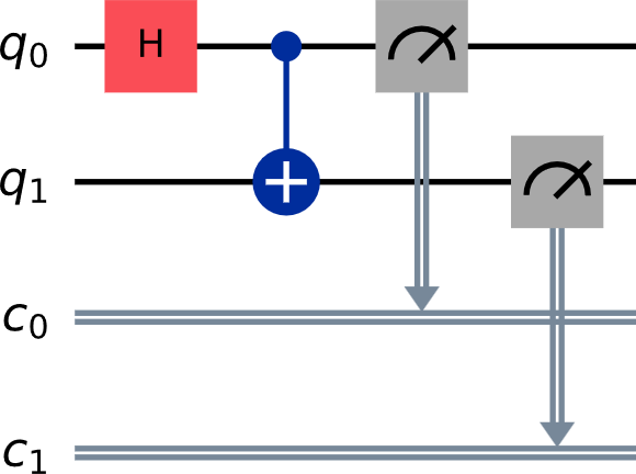
Fig. 1: Quantum circuit with two qubits, two gates and two measurements. A Hadamard gate is applied to the first qubit $q_{0}$ . Then, a CNOT gate is applied to the two-qubit system ( $q_{1}$ and the result of the Hadamard gate being applied to $q_{0}$ ). After this operation, a measurement is performed on each qubit. The results are stored in the classical registers $c_{0}$ and $c_{1}$ .

The Qiskit code corresponding to the quantum circuit in Figure 1 The Qiskit code corresponding to the quantum circuit in Figure 1

quantum_registers = QuantumRegister(2, 'q')
classical_registers = ClassicalRegister(2, 'c')
circuit = QuantumCircuit(quantum_registers, classical_registers)
# apply the Hadamard gate to the first qubit
circuit.h(quantum_registers[0])
# apply the controlled NOT gate for qubit 1 depending on qubit 0
circuit.cx(quantum_registers[0], quantum_registers[1])
# measure both qubits
circuit.measure(quantum_registers[0], classical_registers[0])
circuit.measure(quantum_registers[1], classical_registers[1])

Fig. 2: Result of applying a Hadamard gate and a CNOT gate to two qubits in the state $| 00 ⟩$ – as shown in the quantum circuit in figure 1. The two qubits are measured to be either in the state $| 00 ⟩$ or in the state $| 11 ⟩$ with an equal probability of 50% for each of these two results to be measured.

Exercises

Exercise 1. Check all of the examples listed above—where a gate is applied to one or two qubits—by creating the corresponding quantum circuits. For more information see Programming quantum circuits.

Solution Solution

The quantum circuits must be recreated in the respective environment of the quantum computer, for example using drag & drop. The results will be similar, but probably not identical due to noise.

Exercise 2. Check all of the examples listed above—where a gate is applied to one or two qubits—in a local Qiskit environment. Enter your API token for the IBM Quantum system and run the programmes.

Solution Solution

Here, the quantum circuits must be assembled in Qiskit. To do this, the Qiskit code for the respective example must be incorporated into the general framework.
For the identity gate, for example, a complete programme that can be executed on the IBM Quantum computer (the API token must of course still be added) would then be as follows:

# Create a quantum circuit
from qiskit import QuantumRegister, ClassicalRegister, QuantumCircuit
# Optimise the quantum circuit
from qiskit.transpiler.preset_passmanagers import generate_preset_pass_manager
# Access IBM Quantum
from qiskit_ibm_runtime import QiskitRuntimeService, SamplerV2 as Sampler

service = QiskitRuntimeService(channel="ibm_quantum", token="Insert your API token here, see Profile Settings -> API token")
# Select the least busy quantum computer as the backend
backend = service.least_busy(operational=True, simulator=False)
# Create a sampler connected to the selected backend to run the programme
sampler = Sampler(backend)
# Create a pass manager that will optimise the quantum circuit for the chosen backend; optimisation level 3 is the highest possible level. Lower levels are easier to understand but produce less accurate results
passmanager = generate_preset_pass_manager(3, backend=backend)
quantum_registers = QuantumRegister(1, 'q')
classical_registers = ClassicalRegister(1, 'c')
circuit = QuantumCircuit(quantum_registers, classical_registers)
# Apply the identity gate to the circuit
circuit.id(quantum_registers[0])
# Measurement
circuit.measure(quantum_registers[0], classical_registers[0])

# Create the optimised quantum circuit
optimized_circuit = passmanager.run(circuit)

# Add the quantum circuit as a job to the job queue
job = sampler.run([optimized_circuit], shots=1000)
# Print the Job ID
print("job id:", job.job_id())
# Wait for the results; this can take some time, but the results will also be available on the IBM Quantum platform if the job is interrupted
result = job.result()
print(result[0].data.c.get_counts())

The other examples are analogous, whereby the results will again be similar, but probably not identical due to noise.

Exercise 3. Apply a NOT gate to the superposition states $\frac{1}{\sqrt{2}} \cdot | 0 ⟩ + \frac{1}{\sqrt{2}} \cdot | 1 ⟩$ and $\frac{1}{\sqrt{2}} \cdot | 0 ⟩ - \frac{1}{\sqrt{2}} \cdot | 1 ⟩$ . You can either use matrix notation and bra-ket notation or assemble a quantum circuit or create Qiskit code. Describe the result in your own words.

Solution Solution

$X \cdot (\frac{1}{\sqrt{2}} \cdot | 0 ⟩ + \frac{1}{\sqrt{2}} \cdot | 1 ⟩) = [\begin{matrix} 0 & 1 \\ 1 & 0 \end{matrix}] \cdot (\frac{1}{\sqrt{2}} \cdot | 0 ⟩ + \frac{1}{\sqrt{2}} \cdot | 1 ⟩)$

$= \frac{1}{\sqrt{2}} \cdot ([\begin{matrix} 0 & 1 \\ 1 & 0 \end{matrix}] \cdot [\begin{matrix} 1 \\ 0 \end{matrix}] + [\begin{matrix} 0 & 1 \\ 1 & 0 \end{matrix}] \cdot [\begin{matrix} 0 \\ 1 \end{matrix}])$

$= \frac{1}{\sqrt{2}} \cdot ([\begin{matrix} 0 \\ 1 \end{matrix}] + [\begin{matrix} 1 \\ 0 \end{matrix}]) = \frac{1}{\sqrt{2}} \cdot | 1 ⟩ + \frac{1}{\sqrt{2}} \cdot | 0 ⟩$

$X \cdot (\frac{1}{\sqrt{2}} \cdot | 0 ⟩ - \frac{1}{\sqrt{2}} \cdot | 1 ⟩) = [\begin{matrix} 0 & 1 \\ 1 & 0 \end{matrix}] \cdot (\frac{1}{\sqrt{2}} \cdot | 0 ⟩ - \frac{1}{\sqrt{2}} \cdot | 1 ⟩)$

$= \frac{1}{\sqrt{2}} \cdot ([\begin{matrix} 0 & 1 \\ 1 & 0 \end{matrix}] \cdot [\begin{matrix} 1 \\ 0 \end{matrix}] - [\begin{matrix} 0 & 1 \\ 1 & 0 \end{matrix}] \cdot [\begin{matrix} 0 \\ 1 \end{matrix}])$

$= \frac{1}{\sqrt{2}} \cdot ([\begin{matrix} 0 \\ 1 \end{matrix}] - [\begin{matrix} 1 \\ 0 \end{matrix}]) = \frac{1}{\sqrt{2}} \cdot | 1 ⟩ - \frac{1}{\sqrt{2}} \cdot | 0 ⟩$

In other words, a Pauli-X gate does not change a qubit that is in an equally probable superposition.

Exercise 4. Take the example of a Hadamard gate being applied to a qubit. Explain why it is said that “a measurement reduces the quantum state of a system” (or: “the quantum state collapses”) and why multiple measurements are necessary to obtain a ‘reasonable’ result.

Solution Solution

A qubit to which a Hadamard gate has been applied is in an equally probable superposition of $| 0 ⟩$ and $| 1 ⟩$ . This means that both states are represented simultaneously and that a measurement yielding either $0$ or $1$ is equally probable for both possible outcomes. A single measurement will therefore yield either $0$ or $1$ , but not both or anything in between. However, if multiple measurements are performed, a new quantum system is brought into superposition each time, so that each measurement is taken anew, yielding $0$ or $1$ each time. If many measurements are now carried out (e.g. 1000), on average it is ex-pected that $0$ will be measured approximately 500 times and $1$ approximately 500 times, too (however, it is also theoretically possible that $0$ will be measured 1000 times and $1$ will be measured 0 times, but this is very unlikely).

Exercise 5. Check whether the two qubits described by the state $\frac{1}{\sqrt{2}} \cdot (| 11 ⟩ + | 01 ⟩)$ are entangled. What about two qubits represented by the state $\frac{1}{\sqrt{2}} \cdot (| 01 ⟩ + | 10 ⟩)$ ? Use the method described in Part 3: 2. Entangling two qubits with a Hadamard and a CNOT gate.

Solution Solution

Example 1: $\frac{1}{\sqrt{2}} \cdot (| 11 ⟩ + | 01 ⟩) = \frac{1}{\sqrt{2}} \cdot [\begin{matrix} 0 \\ 0 \\ 0 \\ 1 \end{matrix}] + \frac{1}{\sqrt{2}} \cdot [\begin{matrix} 0 \\ 1 \\ 0 \\ 0 \end{matrix}] = \frac{1}{\sqrt{2}} \cdot [\begin{matrix} 0 \\ 1 \\ 0 \\ 1 \end{matrix}]$

In this case, $a c = b c = 0$ and $a d = b d = 1$ . It follows that $a$ , $b$ and $d$ are equal to $1$ , and $c$ equals $0$ . The superposition state can be written as:

$\frac{1}{\sqrt{2}} \cdot ([\begin{matrix} 1 \\ 1 \end{matrix}] \otimes [\begin{matrix} 0 \\ 1 \end{matrix}])$ ,

which is the combination of two qubit states. The two qubit states are independent of each other; they are not entangled.

Example 2: $\frac{1}{\sqrt{2}} \cdot (| 01 ⟩ + | 10 ⟩) = \frac{1}{\sqrt{2}} \cdot [\begin{matrix} 0 \\ 1 \\ 0 \\ 0 \end{matrix}] + \frac{1}{\sqrt{2}} \cdot [\begin{matrix} 0 \\ 0 \\ 0 \\ 1 \end{matrix}] = \frac{1}{\sqrt{2}} \cdot [\begin{matrix} 0 \\ 1 \\ 1 \\ 0 \end{matrix}]$

In this case, $a c = b d = 0$ and $a d = b c = 1$ . There is no solution that satisfies all the equations (the last two equations are fulfilled if $a = b = c = d = 1$ , but the first two equations require that either $a$ or $c$ , or $b$ or $d$ are equal to $0$ ). This means that the state $\frac{1}{\sqrt{2}} \cdot (| 01 ⟩ + | 10 ⟩)$ cannot be written as Kronecker product of two qubits: The two qubits are entangled.

Exercise 6. Use print(circuit) to print one of the quantum circuits from exercise 1, once before and once after the optimisation step. Describe what you notice. Are there quantum gates that you are not yet familiar with used in the optimisation step? Then research by which matrix they can be represented and what their effect is.

Solution Solution

Firstly, it should be noted that optimisation adapts the quantum circuit to the number of qubits in the quantum computer (while defining many qubits but leaving them untouched). Then, depending on the quantum computer, one or more quantum gates may be replaced by equivalent quantum gates that are available on the quantum computer.
A quantum circuit may also be modified to make it run more reliably. However, the result of the quantum circuit remains the same.

Exercise 7. Use the following code snippet to create and save the quantum circuit as an image (png, svg or LaTeX), once before optimisation and once after optimisation. Describe what you notice. Are there quantum gates that you are not yet familiar with used in the optimisation step? Then research by which matrix they can be represented and what their effect is.

# for drawing circuits
from qiskit.visualization import circuit_drawer

# uses MathPlotLib for creating the graphics; if LaTeX is installed, "latex" could also be used
circuit_image = circuit_drawer(circuit, output="mpl")
# save figure as pixel graphic (PNG)
circuit_image.savefig("Circuit (MPL).png")
# save figure as vector graphic (SVG)
circuit_image.savefig("Circuit (MPL).svg")

Solution Solution

Similar solution as in exercise 6.
For example, the following programme applies a CNOT gate to two qubits, one of which has been brought into superposition by applying a Hadamard gate:

from qiskit import QuantumRegister, ClassicalRegister, QuantumCircuit
from qiskit.visualization import circuit_drawer

quantum_registers = QuantumRegister(2, 'q')
classical_registers = ClassicalRegister(2, 'c')
circuit = QuantumCircuit(quantum_registers, classical_registers)
circuit.h(quantum_registers[0])
circuit.cx(quantum_registers[0], quantum_registers[1])
circuit.measure(quantum_registers[0], classical_registers[0])
circuit.measure(quantum_registers[1], classical_registers[1])

circuit_image = circuit_drawer(circuit, output="mpl", cregbundle=False)
circuit_image.savefig("CNOT.svg")

The result is saved in the file "CNOT.svg".
When optimising, it should first be noted that the optimisation adapts the quantum circuit to the number of qubits in the quantum computer (and in doing so defines many qubits but leaves them untouched). Then, depending on the quantum computer, one or more quantum gates may be replaced by equivalent quantum gates that are available on the quantum computer. A quantum circuit may also be modified so that it runs more reliably, but with the same result. However, the results vary depending on which quan-tum computer is used, because the optimisation is performed for the specific quantum computer in ques-tion.
Since different quantum computers offer different sets of quantum gates, it is possible that very different quantum gates may be applied during optimisation. However, each quantum gate can be represented by a unitary matrix. See list of quantum gates.

Exercise 8. Verify the matrix calculations carried out in the lesson, i.e. for the Pauli-X gate, the identity gate, the Hadamard gate, the CNOT gate, and for the combination of Hadamard and CNOT gates. Compare the theoretical and the measured results – i.e. calculate the squares of the amplitudes representing and, thus, the probabilities of finding the qubit(s) in the different states. Compare these probabilities with the output(s) of the quantum computer.

Solution Solution

It is unrealistic to assume that the exact results will be achieved. However, it will be in a similar range.

Exercise 9 (optional). In addition to the Pauli-X gate, there is also a Pauli-Y gate and a Pauli-Z gate. Research their matrix representations and check their behaviour in a quantum circuit.

Solution Solution

The quantum gates Pauli-Y and Pauli-Z are represented by the following matrices:

$Y = [\begin{matrix} 0 & - i \\ i & 0 \end{matrix}]$ and $Z = [\begin{matrix} 1 & 0 \\ 0 & - 1 \end{matrix}]$ .
The quantum gates Pauli-X, Pauli-Y and Pauli-Z represent reflections on one of the three axes of the Bloch sphere.
In order to visualise the behaviour of these gates in a quantum circuit, use the Quantum Machine.

Exercise 10 (optional). It is possible to replace a quantum circuit by another equivalent quantum circuit (within reasonable approximations). A set of quantum gates that can replace any quantum circuit is called a set of universal quantum gates. Gather information on universal quantum gate sets. Compare quantum circuits that you have run before and after the optimisation. Which universal quantum gate set seems to have been used by the quantum computer?

Solution Solution

Individual answers.

Exercise 11 (optional). Look up various technical possibilities for physically implementing qubits in a quantum computer. Keywords: e.g. superconductors, ion traps.

Solution Solution

Individual answers.

Exercise 12 (optional). In 1996, David P. DiVincenzo introduced criteria for a quantum computer to work. One needs:

Criteria for a quantum computer to work

well-defined qubits;
qubits that are prepared in well-defined initial states;
qubits that are stable for a sufficiently long period of time (decoherence time);
a universal set of quantum gates;
to be able to measure each qubit individually.

Try to explain each criterium using what you have learnt in this lesson. If you get stuck, do some research on the internet.

Solution Solution

A well-defined qubit represents a quantum system that can be manipulated by the gates of the quantum computer. Such a qubit must be initialised in a way that it can be brought in a well-defined state repeatedly. Since qubits can be altered by external influences (including measurements), it is important that they remain stable during a run and can be reliably altered by the gates. The quantum computer must provide a selection of gates that allows all kinds of quantum circuits to be built. Finally, each qubit must be individually measurable. If only some qubits (but not all) can be measured, it is not possible to represent the dependencies between qubits (as is the case with the CNOT gate, for example).

Share this page

Qubits, Quantum Gates and Quantum Circuits – a Computer Science Perspective: Part 3 The CNOT Gate and Entanglement

Context

Content of Part 3

1. The CNOT gate - a gate acting on two qubits

2. Entangling two qubits with a Hadamard and a CNOT gate

Exercises

Criteria for a quantum computer to work

Similar teaching materials

How to implement Deutsch’s algorithm with a Mach–Zehnder interferometer

Careers in Quantum Technologies