Basics of quantum physics

Overview
Overview
Keywords: Quantum state, quantum measurement, quantum entanglement
Age group: 16 – 19
Required knowledge/skills: Students should be familiar, at least to some extent, with the wave phenomena, especially interference; if not, this separately provided optional material can be used: Download 'Interference of waves' as PDF or as docx.
Time frame: 45 min
Author: Aleksandr Sorokin (LV)

Required materials
- Overhead projector – for slides
- Dice of any kind (D6, D12, D20) – for the second activity
Tasks for teachers
- Give an interactive lecture based on the slides (25 min).
- Download the Powerpoint presentation 'Basics of quantum physics' as PPT or as PDF.
- The students do the activities on the worksheet 'Introduction to quantum physics'. Download it as PDF or docx.
- Monitor students’ work, give feedback when needed.
Tasks for students
- Actively participate in the lecture.
- Do the first activity (“States and measurements”) individually, discuss in pairs (10 min).
- Do the second activity (“Modelling a measurement”) in pairs (10 min).
Classically, light is well described as waves: A light beam can reflect from a surface, refract from one medium into another, diffract around obstacles and interfere with another light beam. On the other hand, certain phenomena, such as black-body radiation or the photoelectric effect, cannot be explained within the wave model. In 1900, German physicist Max Planck proposed a revolutionary idea that the black-body radiation problem can be solved if light is thought of as a flux of particles (photons) carrying fixed tiny portions (quanta) of energy, and thus established a wholly new field of quantum physics. The idea that, in different experiments, light can behave either as a wave or as (a flux of) particles is known as particle-wave duality. This duality, as it turned out later, holds for all matter, but is best observed for subatomic-size objects such as elementary particles. If the fact that the same object manifests itself differently depending on the situation still seems paradoxical, think of it in a more abstract way: An object is an entity that can be described mathematically by a quantum state (or a wave function), such that certain mathematical operations on the state determine the behaviour of the object.
Double-slit experiment
Double-slit experiment
One of the classical experiments which demonstrates wave properties of light is the double-slit experiment proposed by British physicist Thomas Young in 1801. In this experiment, monochromatic (‘single-colour’) light illuminates two narrow parallel slits, and on the screen behind the slits, a pattern of bright and dark bands (fringes) is formed.
If we look at the illuminated slits from the standpoint at the screen, we will not see the original source of light, but rather the slits themselves will appear to be the sources. Each of these sources is emitting light waves, which, observed from different points on the screen, will add up (interfere) either constructively – producing a higher light intensity – or destructively – producing a lower light intensity. Hence, the fringe pattern is formed.
Suppose now that, in the double-slit experiment, we gradually reduce the intensity of the incident light beam. It is not hard to guess that the intensity of the fringe pattern on the screen will decrease, while positions and widths of the fringes will stay the same. But what happens if the intensity is so low that, in terms of quantum mechanics, the ‘beam’ contains only a few single photons per second? Intuitively, one might guess that a photon will pass either through one slit or the other, and hit the screen either at the point directly opposite one slit or the other. But reality is slightly different. Although single photons do hit the screen at certain points (and in this respect behave like particles), it turns out that these points can be pretty much anywhere on the screen. The probability to detect a photon at a specific point is maximum where a stronger light wave would form a bright fringe and close to zero where a stronger wave would have a dark fringe (see Fig. 1). Thus, a single photon retains both its particle and wave properties.
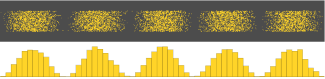
Figure 1
The particle-wave duality was initially thought of as a unique property of light. But come to think about it this way: If light, which classically behaves like a wave, can, in certain experiments, behave like a particle, then why can’t we have it the other way round? Why can’t a particle likewise behave as a wave in some experiments? This idea was theoretically investigated in the 1924 doctoral thesis of French physicist Louis de Broglie, where he introduced the notion of matter waves, suggesting that all matter has wave properties. After three years, clear experimental evidence supporting de Broglie’s hypothesis was found: It was shown that electrons can diffract on a crystal, behaving like waves.
State and measurement
The following section introduces two fundamental concepts: the idea of a state and the role of measurement. These explanations provide the basic understanding needed to grasp how quantum systems behave and how observations affect them.
A system, however big or small it is, can be found in one of several (possibly infinitely many) states. Take the previous example of a single-photon double-slit experiment. After the photon (as a particle) has got to the other side of the plate with the two slits, it is in either of the two states – or [1]– depending on the slit (0 or 1) it has passed through on its way. Classically, the photon must always be exclusively in either state or (known as basis states), but the quantum mechanical description allows us to superimpose the two states as well. The actual quantum mechanical state of the photon after it has passed through the slits is thus the superposition of states and , and can be formally written as , where and are some numbers related to the probability of finding the photon in the corresponding state. More specifically, the probability that the photon has passed through slit 0 is and the probability that it has passed through slit 1 is . As the photon must have passed through either of the slits, .
Photons are not the only particles that can be found in a superposition of states. Pretty much any object – as small as an electron or as huge as a whole Universe – shares this property. For macroscopic systems though, it is close to impossible to distinguish between different states, so quantum effects are best observed for microscopic objects.
In a classical world, we can measure some quantity of a system (say, the length of a table) as many times as we like and the measurement process will not affect the state of the system. In a quantum world, it turns out not to be the case. The result (or outcome) of the measurement is a number (with units, if applicable) that corresponds to one of the basis states. In the previous example, and were two basis states, and the corresponding outcomes might have been, say, 0 (meaning that the photon has passed through slit 0) and 1 (meaning that the photon has passed through slit 1). In the process of measurement, all uncertainty is lost. Suppose the outcome of the measurement is 1. That means that right after the measurement, there is a 100% probability that the system is in state and 0% probability that it is in state . But that would mean that the state of the system has changed from to . We can say that the original state was destroyed, that is, any measurement of a quantum system is destructive.
Hence, there is a major issue. Suppose the system is in the state . In order to estimate the values of coefficients and , the system should be measured several times to gather statistics. The problem though is that you cannot non-destructively measure the system several times, as each measurement will alter and . This issue can at least partly be overcome in a number of ways. The most straightforward one is to prepare several (the more the better) identical copies of the system and then measure them independently. The relative frequency of each outcome (0 or 1) can then be taken as an estimate of squares of magnitudes of corresponding weights ( or ). A physical realisation of this task, though, is far from trivial.
Pure and entangled states
Suppose we have two systems, e. g. two photons – A and B – that have passed through the same double slit. If these photons are independent of one another, then each of them can be described separately with its own state such as
,
,
where and are the states of photon A, while and are the states of photon B. Suppose now that the photons A and B are not independent (or, in common terms, they are entangled), meaning it may no longer be possible to describe photon A separately from photon B. The entangled state of the whole two-photon system can then be written as
,
where etc. are the states which describe the whole system, as opposed to the states , etc., which describe parts of the system separately. Sometimes, to simplify the notation, the indices A and B can be dropped, but then extra care needs to be taken of the order. So, in this simplified notation, the last state can be written as .
As an example, suppose the system of photons A and B is in the state . If we measure just the photon A, and know that it has passed through slit 0, then we immediately know that the photon B has passed through slit 1, and vice versa. This is the idea of an entangled state: measuring only one part of the system gives you at least some information about other parts of the system.
Problems and activities
States and measurements
Format: work individually, discuss in pairs
The system is initialised in the state . If the system is found in the state , the outcome of the measurement is . The system has now been measured.
- Can you determine the outcome of the measurement? Explain.
Suppose the result of this measurement is 0. Another measurement is performed right after the first one.
- Can you determine the outcome of the measurement now?
1000 identical copies of the original system are made and each one is measured once.
- Estimate the number of measurements that will yield 0 and that will yield 1.
- Estimate the mean value of a measurement outcome.
- The probability to measure the system to be in state is , while the probability to measure the system in state is . The result of the measurement is thus non-deterministic.
- The measurement ‘selects’ one of the basis states, in this case , and the original state collapses to , so the probability to measure the system to be in state is , and the probability to measure the system to be in state is . That means that in this particular case, the measurement outcome will deterministically be .
- The probability to measure the system to be in state is and the probability to measure the system in state is [see question 1]. That means that approximately outcomes will be and approximately outcomes will be .
- The mean value by definition is the sum of the products of the outcome and the probability of that outcome. Thus, the mean value of the outcome is .
Modelling a measurement to determine a state
Format: work in pairs
Resources: one or more dice
The system is initialised in the state . The measurement yields 0 if the system is found in state and 1 if it is found in state .
- Student X chooses which faces of a die will correspond to the system measured to be in state and which – to be in state .
- Student Y rolls a die and student X states the result of the measurement. (× 20)
- When enough data are collected, student Y calculates probabilities of each of the two outcomes. Conclude how many die faces your partner has chosen to represent the state and how many to represent the state .
- Discuss: Is the data obtained enough to uniquely obtain coefficients and ? Why or why not?
The ket notation is introduced in the lesson on „Matrices and how they can be used in quantum computing“ .
Share this page