Deutsch’s algorithm - Mathematical approach

Overview
Overview
Keywords: algorithm, Deutsch algorithm
Age group: 16-18 years
Required knowledge/skills: no specific knowledge required
Time frame: 60 minutes
Author: Sergio Rivera Hernandez (DE)
Learning objectives
The goal of this lesson is for students to understand a first example of a quantum algorithm that demonstrates the fundamental structure underlying many quantum algorithms, using a case where the quantum method needs fewer function evaluations than a classical deterministic method. This structure, known as the Golden Circuit pattern, consists of:
- Hadamard gate to create superposition.
- Quantum function evaluation to introduce interference.
- Hadamard gate to close interference.
- Measurement to extract useful information.
At first glance, Deutsch’s algorithm may seem simple, but it encodes the essential principles of nearly all quantum algorithms. The key challenge for the teacher is to present the lesson in a way that makes students appreciate its significance.
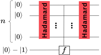
Fig. 1: Hadamard gate
Lesson plan
Before students begin the worksheet, it is crucial for the teacher to emphasize why this algorithm is important. While the problem it solves may appear trivial or unnecessary, the underlying physical principle is the same as in more advanced quantum algorithms—although those require more complex mathematics.
At the end of the lesson, the teacher should explicitly explain how the Golden Circuit pattern will reappear in the upcoming quantum algorithms covered in this course.
| Timing in minutes | Lesson phases | Activity | Material |
|---|---|---|---|
| 0–5 | Introduction | This is a crucial phase of the lesson. The teacher should emphasize that this is the simplest quantum algorithm, the first to solve a problem in a way that a classical computer never could. Despite its simplicity—which allows students to understand every detail—this algorithm exemplifies the fundamental physical principles behind more complex quantum algorithms. This is what makes it so important: If students grasp the basic principles of this algorithm, they will also understand the principles behind other quantum algorithms, as they follow the same foundations. This message should be clearly and explicitly communicated to students. | |
| 5-15 | Work Phase 1 | In this phase, students will receive the worksheet, work on Tasks 1 and 2, and read through the three steps of the algorithm. | Worksheet 2, Tasks 1-2 |
| 15-25 | Intermediate Reflection | In this phase, the results of the first two Tasks will be reviewed to ensure that students have under-stood the general idea before proceeding with the concrete application of the algorithm. | |
| 25-50 | Work Phase 2 | In this phase, students will work on Exercises 3–6. Students who finish early can proceed to using a computer and continue with the next exercises, some of which will be solved using the Quantum Composer. | Worksheet 2, Tasks 3-6 |
| 50-60 | Closure | Discussion of results. In this section, the teacher will once again emphasize the physical principles behind the algorithm and highlight that these prin-ciples will be needed again in the next lesson. Stu-dents should verify that they understand why the quantum algorithm only requires one query, in contrast to the classical case. |
The worksheet deliberately omits normalization factors to keep the focus on the physical principles of the algorithm. Including them could distract students from understanding the core quantum mechanics at play. Teachers should be aware of this when presenting the lesson.
Worksheet 1: Excursion on Quantum Function Evaluation with solutions
The core of quantum algorithms lies in the use of interference, which is one of the fundamental properties of quantum mechanics. This interference is achieved by applying a function f to the entries of the first register. In this lesson, you will learn exactly how this process works.
The following tasks are available as worksheet for download as pdf and docx.
In the worksheet 2, it is assumed that applying the function f introduces a phase shift in the first register in the form
However, this is not explained in detail within the main worksheet 2. For this purpose, Worksheet 1 has been designed to cover Quantum Function Evaluation in full detail.
It is recommended to cover this additional worksheet with the entire group if the students are high-achieving and mathematically inclined. Otherwise, the worksheet can be used as an optional excursion for students or teachers who wish to explore this topic further.

Task 1
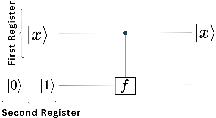
In the first register, you have the state , where x is either 0 or 1. The function f acts as follows:
- If , the states of the second register remain unchanged.
- If , a state in the second register transforms into , and a state into .
The fact that the second register can be transformed according to the value of the function f applied to the first register is represented schematically in the picture above. This is described as the first register controlling the second[1].
Apply the method described above, where the function f acts on the first register and potentially modifies the values of the second register. Complete the following table by determining the values of the second register based on the given function values.
| Function value applied to the first register | Initial state of the second register | Final state of the second register (controlled by ) |
|---|---|---|
| 0 |
| |
| 0 |
| |
| 1 |
| |
| 1 |
| |
| 0 |
| |
| 1 |
|
| Function value applied to the first register | Initial state of the second register | Final state of the second register (controlled by ) |
|---|---|---|
| 0 |
|
|
| 0 |
|
|
| 1 |
|
|
| 1 |
|
|
| 0 |
|
|
| 1 |
|
|
Task 2
In this task, you will use the results from Task 1 to understand the key trick used in quantum algorithms to introduce interference, which is the core of quantum computing. Quantum algorithms use the following circuit for a function that acts on the first register while controlling the second register.
a) Show that if , then the full state
remains the same.
b) Show that if , then the full state transforms
transforms into
and that this can be written as:
c) Justify that the results from a) and b) are contained in the following general expression:
Step 1: Showing that if , the full state remains the same
We start with the initial state:
- Since , the function does NOT flip the second register.
- The second register remains in its original state: .
- Thus, the full state remains unchanged:
Conclusion: The state is NOT affected when .
Step 2: Showing that if , the state transforms
We start with the same initial state:
- Since , the function flips the second register:
- →
- →
- Applying this transformation results in:
- which is equivalent to introducing a phase factor:
Conclusion: When , the state gains a phase factor of .
Step 3: Justifying the General Expression
From the previous two steps, we observe:
If : (no change)
If :
This pattern can be summarized in the generalized form:
Conclusion: This means that the second register remains completely unchanged, but the first register gains a phase factor of .
Final Conclusion: The Role of Quantum Function Evaluation in Quantum Algorithms
In this lesson, you learned how quantum function evaluation introduces interference, the core mechanism behind quantum algorithms. Instead of simply modifying a qubit’s state, the function encodes information in the phase of the first register.
The state in the second register is crucial for achieving this interference. It ensures that function evaluation does not store information classically but instead modifies the phase of the first register.
Since this phase encoding is present in most quantum algorithms, understanding it is essential for both the mathematical formulation of quantum computing and its practical implementation in tools like Quantum Composer or Qiskit. Mastering this principle will help you understand how quantum circuits solve problems more efficiently than classical algorithms.
Worksheet 2: Deutsch’s Algorithm with solutions
The following tasks are available as worksheet for download as pdf and docx.
Deutsch's algorithm, developed by David Deutsch in 1985, marks a significant milestone in the world of computing. It's the first instance where a quantum algorithm showed a potential advantage over classical algorithms. This discovery opened the door to the idea that computers based on the principles of quantum mechanics could solve certain types of problems more efficiently than classical computers.
In this lesson, you will learn how Deutsch's algorithm works. To fully grasp its significance, you'll first need to understand how the problem the algorithm solves can be approached using classical computing methods.
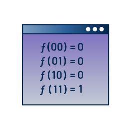
The Problem
Imagine we have a mystery box represented by a function . This box is special because when you give it a number (either 0 or 1), it gives you back a number (also either 0 or 1). But there's a secret about how our box works, and we want to find out what it is.
The box works in one of two ways:
| Constant functions | Balanced functions | ||
|---|---|---|---|
|
|
|
|
Our challenge is to figure out if our mystery box (function ) is constant or balanced by asking it questions, that is, by giving it numbers (0 or 1) and seeing what it returns.
Classical Solution
Task 1: Describe the main difference between a constant function and a balanced function.
Task 2: Determine the minimum number of questions you need to ask the box to find out whether the function is constant or balanced. Justify your answer.
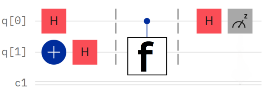
The Deutsch algorithm tackles our problem using just one query, thanks to the power of quantum computing. It employs the following quantum circuit
that operates in three main steps, utilizing quantum bits (qubits) and quantum gates. Here's how it's set up:
For the first qubit (in our first register), we start with the state . For the second register, we use the special combination of states − . The algorithm unfolds in three key steps:
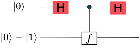
Step I: Apply a Hadamard gate to to create an equal superposition of and .
Step II: Apply the function , which modifies the phase of the first register according to . This step is crucial for quantum interference. If you would like to explore where this phase factor comes from in more detail, see the optional worksheet on quantum function evaluation.
Step III: Apply a Hadamard gate again to the first register. This step interferes the phase‑modified states, allowing measurement to determine whether is constant or balanced.
Your Task: Understanding Step by Step
Now, you will delve into each step of the algorithm to understand how quantum principles enable solving the problem with a single query.
Task 3, Step I: Explain why the input state transforms into the state after applying the first Hadamard gate.
Hint: The Hadamard operator can be expressed as . Note that the result is considered up to an irrelevant overall factor.
Task 4, Step II: In this step, by using quantum function evaluation to introduce phase shifts in the first register, it can be shown (see WS on quantum function evaluation) that the state transforms into:
a) Demonstrate that for a constant function , the state simplifies to , up to an irrelevant overall factor.
b) Demonstrate that for a balanced function , the state simplifies to , up to an irrelevant overall factor.
Task 5, Step III: In this step, you will apply the Hadamard gate to the states obtained in Task 4.
a) If the function is constant, apply the Hadamard gate to the state and show that you obtain the state .
b) If the function is balanced, apply the Hadamard gate to the state and show that you obtain the state .
Task 6
a) Which state do you measure after Step III if the function is constant? ______
b) Which state do you measure after Step III if the function is balanced? ______
c) Explain how your answers in a) and b) effectively solve the problem.
Implementation with the Quantum Composer
The Deutsch Algorithm can be easily implemented using the Quantum Composer with the following circuit:
In the following tasks, you will model and test the algorithm with the quantum composer.
Task 7: First, you need to model the constant and balanced functions using the quantum composer. These functions can be represented using specific configurations of quantum gates.
Consider as the input qubit (the x-value of ) and observe how the value of the second register changes after applying the gates specified. The final state of the second register represents the output of .
Below are the gate configurations for the functions , , and . Each configuration corresponds to one of these functions:
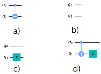
Match each of the functions , , and with the correct circuit.
Task 8: Explain why the following part of the circuit
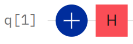
results in the state .
Task 9: Now, you're ready to experiment with the quantum composer. Choose one of the representations of the functions , , or , implement the circuit in the quantum composer, and verify if the algorithm works as expected.
Task 1: Difference Between Constant and Balanced Functions
Constant function: Outputs the same value for all inputs (either always 0 or always 1).
Balanced function: Outputs 0 for one input and 1 for the other.
Task 2: Minimum Number of Queries (Classical Case)
Classical computing requires 2 queries to determine if the function is constant or balanced.
Task 3: Applying the Hadamard Gate in Step I
- The Hadamard gate creates superposition:
- Applying H to transforms it into (up to normalization).
Task 4: Phase Encoding via Function Evaluation in Step II
- For a constant function f(x): ~ (no phase difference).
- For a balanced function f(x): ~ (introduces a phase shift).
Task 5: Applying the Hadamard Gate Again in Step III
- If f(x) is constant:
- If f(x) is balanced:
Task 6: Measurement Outcome
- If the function is constant: is measured.
- If the function is balanced: is measured.
By using superposition, the quantum program can determine whether the function is constant or balanced with just one evaluation of the function. A classical deterministic method needs two evaluations, because it has to check both input cases separately.
What makes this especially remarkable is that distinguishing between “constant” and “balanced” is a global property of the function. That means: you cannot recognize it by looking at a single input-output pair. Only by comparing both values, and , can you decide. A classical algorithm must therefore query both values separately.
In contrast, a quantum algorithm like the Deutsch algorithm uses superposition and interference to evaluate both inputs simultaneously. This allows it to analyze the global structure of the function in a single computational step. The measurement process then yields exactly one bit of information, which directly reveals the sought-after global property.
The Deutsch algorithm also illustrates two important points:
- Quantum computers are not superior in every respect.
The quantum algorithm only decides whether a function is constant or balanced—it does not identify the exact function in the black box. Whether a given problem is suitable for quantum computing must be analyzed on a case-by-case basis. - The solution lies in the input qubit.
In the end, it is not the output qubit but the input qubit that is measured. During the algorithm, the relevant information is “moved” into this qubit, while the other part of the system loses information. Such information shifts are typical in many quantum algorithms. Often, the solution lies in places we would not intuitively expect.
Although the Deutsch problem is a rather simple and theoretical construct, it was the first to demonstrate fundamental principles of quantum computing. It paved the way for more powerful quantum algorithms that will be explored in the following lessons.
Final Conclusion
- The second register is never affected; only the phase of the first register changes based on .
- This phase encoding is essential for quantum interference, which is the foundation of quantum speedups.
Mathematically, this operation corresponds to a so-called controlled modulo-2 addition (XOR operation), which can be expressed as follows:
Here, denotes addition modulo 2. This means:
If , the state of the second qubit is flipped ().
If , the state remains unchanged.All images are screenshots taken from IBM Quantum Composer.
Share this page